How to read the math in arXiv AI papers: a practical guide

Reading the mathematics in an AI paper is a useful skill for engineers who need to understand a model, reproduce a method or assess an experimental claim. This guide explains how to decode the notation, check an equation on small numbers and connect it to the surrounding paper and implementation. It assumes you can read code, but does not assume that research notation is already familiar.
An equation compresses several decisions into one line: the objects being manipulated, their dimensions, which values are sampled, and what is learned or held fixed. Recovering those details is a good first step. Explaining why a method works and implementing it faithfully take further work.
Start with the attention walkthrough: it connects one equation to array shapes, small numbers and runnable Python. The notation reference explains the expressions you will meet in other papers. The rest of this series applies the same method to equations from specific papers: architecture equations such as RoPE, MLA and LoRA; training objectives such as DPO and GRPO; and generative models and metrics such as the ELBO, diffusion and pass@k. Those parts come out on 4, 5 and 6 November; until then, the walkthroughs this part refers to are not linked. For a longer treatment of the foundations, Tianhua Chen’s The Little Book of Generative AI Foundations develops the linear algebra and probability behind generative models.
Attention, read one symbol at a time
Attention produces an output vector by taking a weighted average of value vectors. It obtains the weights by comparing a query vector for the output position with a key vector for each available input position. The matrices , and collect those query, key and value vectors. Scaled dot-product attention combines these steps in equation (1) of §3.2.1 (§ means “section”) in Attention Is All You Need:
The definitions are in the text, not in the equation. The paragraph before equation (1) says that queries and keys have dimension and values have dimension . The method takes the dot product of each query with all keys, divides each by and applies a softmax “to obtain the weights on the values”. Queries are “packed together into a matrix ”, and keys and values into and . So each row of these matrices is one token’s vector, and the softmax produces one set of weights per query. The learned matrices that turn token vectors into , and appear later, in §3.2.2.
Shapes and roles. An attention head performs one such calculation with its own query, key and value vectors. Write down their shapes before reading the operators. For one head with queries and keys:
| Symbol | Shape | What it is | Where it comes from |
|---|---|---|---|
| one query row per output position | token vectors times a learned matrix | ||
| one key row per position that can be attended to | token vectors times a learned matrix | ||
| one value row per key | token vectors times a learned matrix | ||
| transposed: rows become columns | the same numbers as | ||
| a number | the width of each query and key | a fixed setting: 64 in the base Transformer |
Papers give a shape by naming the set the matrix belongs to: means a matrix of real numbers with rows and columns, an array of shape [n, dk].
Read from the inside out.
-
multiplies an matrix by a matrix. The shared is summed away, so the result is an table of scores. Entry is the dot product of query and key : multiply corresponding entries, then add the products. For fixed vector lengths, this score is larger when their directions are more similar.
-
Dividing by stops the scores from growing with the vector width. Footnote 4 of the paper shows why unscaled dot products grow. Suppose the components of a query and a key are independent of one another (knowing some of them tells you nothing about the others), each with mean 0 and variance 1 (the average squared distance from the mean). Then:
The lines use two rules about independent numbers. First, the product of two independent numbers that each have mean 0 and variance 1 also has variance 1. Second, when independent numbers are added, their variances add, so the products give variance . The standard deviation is the square root of the variance, . Dividing every score by shrinks the spread by the same factor, back to 1.
Why the two rules hold
Variance when the mean is 0. Variance is the average squared distance from the mean. When the mean is 0, the squared distance from the mean is just the square of the number, so the variance is the average of the square. A component with mean 0 and variance 1 therefore has averaging 1.
The average of a product. For independent numbers, the average of a product is the product of the averages. Take a number that is 1 or 3 with equal chance, so it averages 2, and a number that is 1 or 5, also with equal chance, so it averages 3. Independent means that takes each of its values equally often whatever turned out to be, so all four pairs are equally likely. When , the products are 1 and 5, which average . When , they are 3 and 15, which average . Either way the average is , so over both values of it is , which is . Without independence the rule fails: if were 5 whenever is 3, and 1 whenever is 1, only the products 1 and 15 would occur, and they average 8. Wikipedia states the rule for any independent random variables, with “expected value” for the average: independence and expectation.
Rule 1: one product has variance 1. Take one product . Its mean is the product of the averages, , so its variance is the average of . The squares are independent because and are, and each averages 1, so the variance is . The general formula is the variance of a product of independent variables.
Rule 2: the variances of independent terms add. Call the products , so the dot product is the sum . The terms are independent because each uses different components, and each has mean 0 and variance 1. The sum has mean 0 too, so its variance is the average of its square. Multiplying the sum by itself gives one product for every pair of terms, a grid:
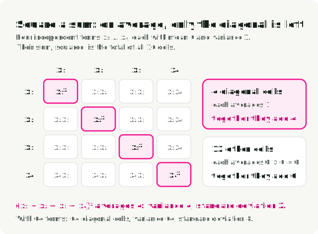
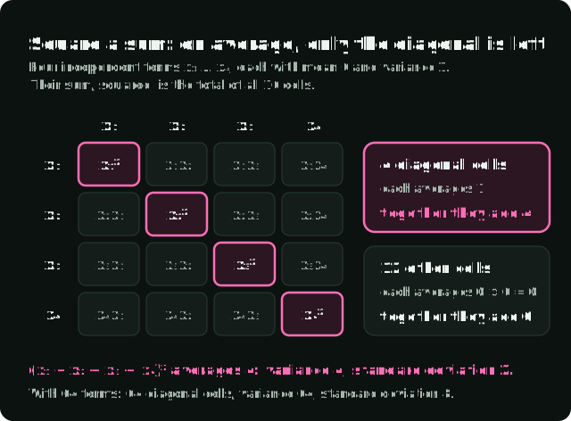
The diagonal cells are the squares , and each averages 1. Every other cell multiplies two different, independent terms, so its average is the product of their averages, : its positive and negative values cancel. Only the diagonal cells are left, so the variance of the sum is and its standard deviation is . The spread grows with the square root of the width because most of the grid cancels out. Wikipedia gives the general statement as the variance of a sum of uncorrelated variables; independent variables are always uncorrelated, so the rule covers them.
With , raw scores typically spread over about ; scaled, over about , at any width.
Widely spread scores saturate softmax (step 3), and its gradients vanish. If one score in a row is far above the others, softmax gives that key a weight near 1 and every other key a weight near 0. A small change to any score then barely moves the weights, so the gradient that reaches the queries and keys is close to zero, and training has almost nothing to adjust them with. The paper offers this as the likely explanation of an earlier result: without the scaling, dot-product attention did worse than additive attention, an older form that scores a query and a key with a small network, at large (Britz et al., 2017). The paper does not measure the gradients itself.
-
Softmax turns each row of scores into weights. Let be one row of the scaled scores. The exponential , also written , uses the constant . Then , where is just a second index name, so the sum runs over every key in the row. The weights are positive and each row sums to 1.
-
Multiplying the weights by the values sums away the key axis. Row of the output is a weighted average of the value rows, weighted by how well each key matched query .
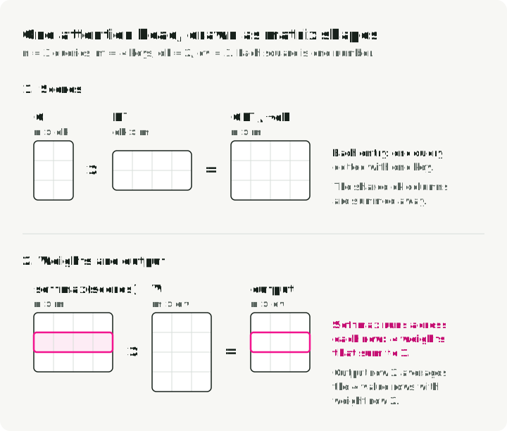
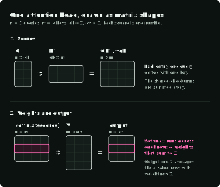
Count the squares in the figure: each product removes the axis its two grids share.
Check it with two numbers. Take one query and two keys whose scaled scores are , chosen so that the exponentials come out as 1 and 3, and values and . The figure works through it one operation per column:
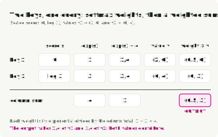
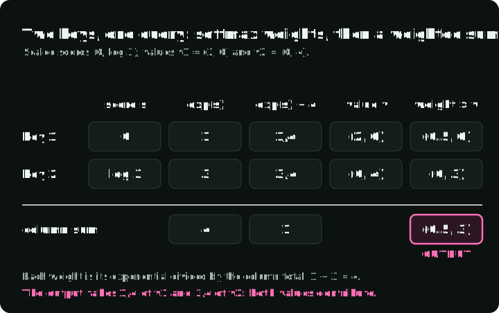
Attention blended both values; it did not pick the better-matching token.
Compare it with code. The NumPy function below implements one head. k.T is the transpose. axis=1 is the key axis, so each query’s row is normalized separately. The row maximum is subtracted before np.exp: adding the same number to every score in a row cancels in the softmax ratio, so the result is unchanged, but large scores no longer overflow. The optional mask sets blocked scores to , which makes their weights exactly zero. A decoder uses such a mask to stop each token from attending to later tokens (§3.2.3 of the paper).
Save the block as attention_example.py and run uv run --with numpy python attention_example.py. The checks pass silently.
import numpy as np

def attention(q, k, v, allowed=None):
    """One head. q: [n, dk], k: [m, dk], v: [m, dv], allowed: bool [n, m]."""
    scores = q @ k.T / np.sqrt(q.shape[1])  # [n, m]
    if allowed is not None:
        if not allowed.any(axis=1).all():
            raise ValueError("every query needs at least one allowed key")
        scores = np.where(allowed, scores, -np.inf)
    scores = scores - scores.max(axis=1, keepdims=True)
    weights = np.exp(scores)
    weights = weights / weights.sum(axis=1, keepdims=True)  # rows sum to 1
    return weights @ v, weights  # [n, dv], [n, m]

# The two-key example from the text.
out, w = attention(
    np.array([[1.0]]),
    np.array([[0.0], [np.log(3.0)]]),
    np.array([[2.0, 0.0], [0.0, 4.0]]),
)
np.testing.assert_allclose(w, [[0.25, 0.75]])
np.testing.assert_allclose(out, [[0.5, 3.0]])

# A causal mask: query i may attend only to keys 0..i.
x = np.random.default_rng(0).normal(size=(3, 4))
out, w = attention(x, x, x, allowed=np.tril(np.ones((3, 3), dtype=bool)))
assert out.shape == (3, 4)
np.testing.assert_allclose(w.sum(axis=1), 1.0)
assert np.all(w[np.triu_indices(3, k=1)] == 0)
A query whose keys are all blocked is a case the equation leaves open: every weight in its row would be . The function raises an error instead of returning NaN.
From one head to several. The base Transformer runs eight heads in parallel, each with its own learned matrices for producing , and , and each with . It concatenates their outputs and multiplies the result by another learned matrix, (Attention Is All You Need, §3.2.2).
An implementation can also process a batch: several input sequences together. For example, PyTorch’s scaled dot-product attention accepts a query tensor Q with shape [batch, heads, n, d_k]. The first two dimensions select a sequence and a head; Q[b, h] is the [n, d_k] matrix for that pair. The attention formula applies separately to each pair. The NumPy function here handles only one such pair: its .T and axis=1 operations assume two-dimensional inputs.
Six questions for any equation
| Question | Answer for attention |
|---|---|
| What does the equation return, and with what shape? | An matrix: one output row per query |
| Is each symbol data, a trained weight, a frozen model, a setting or a sample? | , and are computed from tokens by learned matrices; is a fixed setting; nothing is sampled |
| Over which index or axis does each operation run? | Softmax runs over the keys in each query’s row; the product of the weights with sums over keys |
| Where are the definitions? | The paragraph before equation (1), footnote 4, and §3.2.2 for the learned projections |
| What does a check with two or three numbers give? | Weights and output |
| What did the code have to decide that the equation leaves open? | Subtracting the row maximum, the value used for masked scores, a row with no allowed key |
What kind of statement an equation makes
Attention is a computation: it says how to get an output from inputs. Papers also write equations that do other jobs:
| Kind | Example in this series | What to check |
|---|---|---|
| Computation | The attention output; MLA’s compressed vector | The shape of every intermediate result |
| Definition | GRPO’s score relative to other answers | What the new name stands for, so you can substitute it back |
| Objective: a loss to minimize or a score to maximize | The DPO loss | Whether it is minimized or maximized, and which data it averages |
| Update rule | Gradient descent; Gated DeltaNet’s memory | What changes at each step and what stays fixed |
| Constraint, or a set of allowed values | mHC’s allowed mixing matrices | How the paper produces a value that satisfies it |
| Bound: an upper or lower limit on a quantity | The evidence lower bound (ELBO) | The difference between the two sides, and when it is zero |
| Estimator or metric | pass@k | What is counted, and from how many samples |
| Empirical fit | DeepSeek LLM’s scaling law | The range of data the curve was fitted on |
A constraint states a property the result must have. For attention weights, that property is: every weight is nonnegative and each row sums to 1. Softmax is a computation that produces weights with that property. The requirement alone does not tell you to use softmax.
asserts that two expressions are equal. means “is defined as”: it gives a name to an expression. A definition can name a metric, a loss or a set of allowed values, so seeing does not tell you which kind of equation in the table above you are reading.
For example, Evaluating Large Language Models Trained on Code, the paper that introduced the Codex code-generation model, uses to define its estimator for pass@k (equation 1). This metric measures the chance that at least one of generated programs passes the tests. In the DeepSeek-V4 technical report, equation (2) combines two statements: defines a set of allowed matrices, and requires the model’s mixing matrix to belong to that set. The definition uses ; the constraint uses , meaning “belongs to”. The pass@k and mHC sections work through those examples.
Finding the new equation, its definitions and its code
A paper’s methods section describes how its model or training algorithm works. The heading may be “Method”, “Architecture” or something more specific. Authors often explain an existing method first, then show what they changed. To identify the claimed contribution, start with the introduction’s summary of what is new. For example, DeepSeekMath, §1.1 lists Group Relative Policy Optimization (GRPO), its method for training models from scored answers. Section and equation numbers here refer to the linked paper.
Then compare the proposed method with the earlier method it changes. Two papers illustrate this:
- An architecture change. DeepSeek-V2 describes standard multi-head attention in §2.1.1 and introduces multi-head latent attention (MLA) in §2.1.2. Standard attention stores every earlier token’s keys and values. MLA stores a compressed vector from which they can be reconstructed. Comparing those equations reveals what the model stores differently; the MLA walkthrough derives the memory saving.
- A training change. DeepSeekMath, §4.1.1 prints the objective of Proximal Policy Optimization (PPO) as equation (1) and GRPO as equation (3). Both use an advantage: a number that says whether an answer was better or worse than expected. PPO estimates it with a second learned network, the value model, which predicts the reward still to come from a partial answer. GRPO instead compares the answer’s reward with rewards for other answers to the same question. The GRPO walkthrough compares these terms using the whole-answer notation from DeepSeek-R1.
Find the definitions around the equation. Check the preceding paragraph, any “where …” sentence after it, footnotes and appendices. In Attention Is All You Need, the paragraph before equation (1) defines the dimensions, and footnote 4 explains the scale factor. DeepSeek-V3 defines most of its routing symbols right after equation (15), and the bias just before equation (16). DeepSeek-V2 develops MLA across equations (9)–(19), then collects the computation in Appendix C.
Check the algorithm and code. An algorithm box is a numbered pseudocode listing that gives the order of operations. DeepSeekMath’s Algorithm 1 shows when to generate answers and when to update the model. Algorithm 1 in Denoising Diffusion Probabilistic Models (DDPM) specifies how to sample the training image, noise level and noise. Implementations settle further details: by default, np.std divides the sum of squared deviations by , while torch.std divides by . The GRPO example shows how that choice changes the advantage values computed from the same rewards.
arXiv versions can move sections and repeat equations under new numbers, so cite the version. In DeepSeek-R1 v1, the GRPO objective is §2.2.1, equations (1)–(3). In v2, posted in January 2026, it is §2.1, and the same equations reappear as (11)–(13) in Supplementary A.3. A link without a version opens the latest one, so every arXiv link in this series includes the version it was checked against.
Checking your reading with an LLM
A chat model can draft the symbol table, the index of every sum and a small-number check, if you give it the definitions and ask it to flag what is missing. Text copied from a PDF flattens subscripts, superscripts and fractions into one line; the “HTML (experimental)” and “TeX Source” links on the arXiv abstract page give clean text to paste. Paste the equation and the paragraphs around it with a prompt like this:
Below is equation (N) from <paper title, arXiv ID and version>, followed by
the paragraphs that define its symbols.

1. Make a table with one row per symbol: shape or type, meaning, and whether
   it is input data, a trained weight, a frozen model, a fixed setting or a
   random sample. Quote the sentence that defines it.
2. List every symbol the pasted text does not define. Do not guess them.
3. For every sum, mean, softmax, min or expectation, name the index or the
   distribution it runs over.
4. Work through the equation with the smallest numbers that use every term.
5. Say which kind of statement it is: a computation, definition, objective,
   update rule, constraint, bound, estimator or empirical fit.
Without step 2, nothing stops the model from filling a missing definition with the letter’s usual meaning, such as reading in DPO as a standard deviation instead of the sigmoid. The quotes from step 1 make the table checkable: search the PDF for each one, and treat a row whose quote you cannot find as a guess.
The same procedure as agent skills. paper-math-skills packages this section and the notation reference below as two skills written for Claude Code; other agents that load SKILL.md files can use them too. read-paper-math fetches the pinned arXiv version, quotes the sentence that defines each symbol, reads the equation from the inside out and runs a small-number check. check-paper-math reviews such a reading against the paper: it searches for every quote, re-runs the numbers and flags claims stronger or weaker than the paper’s. paper-math-readings has the skills’ readings for Parts 2–4, one for each of the 15 sections with a Source: line.
Notation reference
If a Greek letter is unfamiliar, open this article’s Greek-letter reference (Appendix A) for its name and common meanings. For more practice with the mathematics, Stanford CS229 provides probability and linear algebra reviews with exercises; Dive into Deep Learning’s preliminaries explain the foundations with code.
Subscripts, marks and relation signs
Letters are local variable names: each paper defines its own. Subscripts are usually indices. may be coordinate of a vector or example in a dataset, and is the model’s vector for token , called its hidden state.
Superscripts in model papers are often labels. In , the superscript in parentheses is usually a layer number, not a power; in DeepSeek-V3’s and it marks shared and routed experts, the ones every token uses and the ones a router picks (see the MoE routing example). In DeepSeek-V2, and carry labels, not exponents; the MLA example defines those labels. is a transpose and is a square.
means positions 1 through , including , unlike a Python slice; papers usually count from 1. means every position before . selects row , as in NumPy slicing.
Marks on a letter usually change its meaning in one of these ways:
| Mark | Usual reading | Example or exception |
|---|---|---|
| A prediction or an estimate | Example: in DeepSeekMath estimates how much better an answer scored than expected | |
| A mean | Exception: in DDPM, multiplies the noise schedule’s factors from step 1 through | |
| A perturbed or unconstrained version | Example: in DeepSeek-V4, is a matrix before normalization enforces its constraints | |
| The optimum | Exception: in DPO, is the true reward, which the method never observes | |
| A new value or an intermediate | Example: in DeepSeek-V3, is an expert weight before normalization | |
| The matrix inverse | Not the entrywise reciprocal: undoes , (the identity matrix), and in general |
Some symbols other than Greek letters also have several jobs:
| Symbol | Meanings |
|---|---|
| Conditioning in ; “such that” inside a set | |
| An absolute value; the length of a sequence, as in , the token count of GRPO’s answer ; the size of a set | |
| ”Is sampled from” in ; “roughly” in informal text | |
| A sequence length; a softmax temperature; the number of diffusion steps | |
| A query vector (attention); a question (GRPO); the student model (distillation); the encoder (ELBO) |
Five signs say how two sides relate. , sometimes , defines a new name. marks an approximation, such as the sampled average in Expectations and where the samples come from. means “proportional to”, with a normalizing constant left out: becomes a distribution only after dividing by . means “much smaller than”, as in DeepSeek-V2’s : the compressed width is much smaller than the total width of all heads. is an assignment, as in an update rule.
Sums, counts, intervals and logarithms
The large adds terms and multiplies them. The index below each operator starts at 1 here and runs through the upper limit :
The index belongs to the operator, as a loop variable belongs to its loop. In , the sum runs over , while identifies an output entry. The result is a vector with one entry per : the matrix-vector product written out. The indices on the left-hand side tell you the shape of the output.
The factor in front of a sum decides what gets equal weight. A batch with a 2-token answer and an 8-token answer, where is the loss on token of answer (in GRPO, is a term to maximize instead), can be averaged in two ways:
In the first, each answer gets weight , shared among its tokens:
In the second, every token has weight . GRPO samples answers to each question, and is the number of tokens in answer . The two averages then read as follows, for DeepSeekMath’s GRPO and for DAPO, a later variant of GRPO:
With , these are and above. DAPO switched to the per-token average (§3.3) because the per-answer average gave the tokens of long answers too little weight: the model learned too little from long good answers and did not penalize long, repetitive bad ones enough.
A sum can also count. Papers do this with an indicator: a bold one followed by a condition, , which equals 1 when the condition is true and 0 when it is false. Some papers put the condition in parentheses or print a double-struck one instead; the meaning is the same. Adding up indicators therefore counts how many times the condition holds. Accuracy is the usual example. If is the predicted class and the correct class for example , then is the number of correct predictions. Predictions (cat, dog, dog) against correct labels (cat, cat, dog) give the indicators 1, 0 and 1, so the count is 2 and the accuracy 2/3. In a mixture-of-experts (MoE) layer, a router sends each token to a few of many feed-forward sub-networks, called experts. In DeepSeek-V3’s balance loss (equation 18), the indicator is 1 when an expert’s score for a token is among the highest scores for that token, where is how many experts each token is routed to. Its sum over the tokens of a sequence counts how often that happened. The score here leaves out the bias that routing adds, so the count can differ from the experts the router actually picks (MoE routing).
The binomial coefficient , read ” choose ”, counts the ways to choose distinct items from without regard to order. For integers , it equals . The exclamation mark means factorial: , with . For example, : five items have ten distinct pairs. DeepSeekMoE uses binomial coefficients to count expert combinations, and the pass@k estimator uses them to count sets of samples.
Intervals use brackets for included ends: includes both, neither. In Gated DeltaNet, means strictly between 0 and 1. Elsewhere, is a pair.
The natural logarithm reverses exponentiation: . Logarithms turn products into sums and ratios into differences: and , but does not split. That is why papers work with log-probabilities. The log of a product of token probabilities is a sum, and the log of a ratio of two models’ probabilities is a difference, the form used in the DPO and GRPO objectives. ML papers mean the natural log unless they say otherwise; the results are in nats, and base-2 logs give bits. For a probability , , and it grows without limit as approaches 0, so a confident wrong prediction is expensive.
Log-sum-exp means: exponentiate each score , add the results, then take the logarithm. Computing directly can overflow when a score is large. Instead, find the largest score and call it . The notation means “compare all entries and take the largest one”; in NumPy, m = z.max().
Subtract from every score before exponentiating, then add it back after taking the logarithm:
For , the largest score is . The shifted scores are , so the calculation becomes . Neither exponential is larger than 1. The attention code uses the same subtraction before softmax; there the common factor cancels in the division, so nothing is added back.
Conditional probability and the probability of text
is the probability that the model with parameters assigns to output given input . The subscript names the parameters; some papers write , where the semicolon also marks parameters rather than a condition. With a dot in place of the output, is the whole distribution over outputs rather than one number. RL papers write the same object as , the probability that the model writes answer to question , and call the model a policy.
Swapping the event and the condition gives a different number. Suppose 100 model responses: 60 are correct, 50 are valid JSON, and 40 are both. Then
Let mean “the response is correct” and mean “the response is valid JSON”. Conditional probability restricts the count to responses satisfying the condition: , provided . The symbol means “both events happen”. Here the fraction is , the same as 40 correct responses among 50 valid-JSON responses.
Two events are independent when knowing that one happened does not change the probability of the other. That requires . In this sample, , while , so the observed proportions do not satisfy independence.
Bayes’ theorem, also called Bayes’ rule, relates the two directions of conditioning: . It lets you compute the probability of given from the probability of given and the probabilities of the two events. The ELBO example uses it to find the probability of a hidden code given an observed image.
A language model scores a sequence one token at a time. By the chain rule of probability,
Each factor conditions on every earlier token, so the formula does not assume tokens are independent. If three tokens have conditional probabilities 0.5, 0.2 and 0.1:
The usual training loss is the negative of this sum, divided by the length:
During training, the earlier tokens come from the dataset. During generation, they are the model’s own earlier choices.
Expectations and where the samples come from
An expectation is a probability-weighted average:
Read as “the average of when is drawn from ”. The notation sums over all possible discrete values of . Without a subscript, averages a random variable over its own distribution: if is 1 with probability 0.75 and 3 with probability 0.25, then .
When a variable has a density , meaning probability per unit of , the weighted average is an integral, . The identifies as the variable being integrated; with no limits written here, the integral covers its whole range. The density example explains probability per unit and shows an integral as an area under a curve.
Training code cannot sum over every possible input, so it samples and averages: , with each drawn independently from , which papers write as . Papers call this a Monte Carlo estimate, and in code it is loss.mean() over a batch. The batch mean estimates the expectation only if the batch is drawn from the distribution in the ‘s subscript, so the subscript tells you how the training data is produced:
- DPO averages over saved examples : a prompt, a preferred answer and a rejected answer. The answers are collected and labeled before this training stage; they may come from earlier model generation. At each training step, the model computes probabilities for those supplied answers and updates its weights. It does not sample fresh answers for that step.
- GRPO in DeepSeek-R1: generate answers, then compare their rewards. Training draws a question from the dataset, generates several answers, and scores them with a reward function, such as checking a mathematical result or running unit tests. The update favors answers that scored above the group’s average. The notation means “sample a question from the question distribution”. The notation means “sample answers to that question from the model copy named ”. The subscript old marks the copy that generated these answers; that copy stays fixed while the batch is used for updates. The GRPO walkthrough explains the reward comparison and updates.
- On-policy distillation in MiniLLM and DeepSeek-V4: generate text, then learn from teacher probabilities. The model being trained is the student. It generates text; a frozen teacher supplies next-token probabilities for the same prefixes, and training adjusts the student’s probabilities toward the teacher’s. These probabilities provide the training signal, rather than GRPO’s reward score for an answer. MiniLLM writes student-sampled text as : is the text and names the student model. DeepSeek-V4 calls its student and uses several specialist teachers. MiniLLM’s actual sampling procedure also mixes in tokens drawn from the teacher. The distillation walkthrough explains the objectives and that sampling distinction.
The order tells you what training optimizes. Suppose a model assigns probabilities 0.9 and 0.1 to the correct outputs of two equally weighted training examples. Averaging their log-probabilities means taking each log first, then averaging: np.log(probs).mean(). Taking the log of their average means np.log(probs.mean()). If is the probability assigned to a randomly chosen example’s correct output:
Negating these scores gives losses of 1.20 and 0.69. A second model that assigns 0.5 to each correct output gets 0.69 under either calculation. Thus averaging probabilities before taking the log treats the two models as equally good, while the usual average negative log-probability penalizes the first model more for its low probability on the second correct output. When translating a loss into code, preserve the order of the log and the average.
Jensen’s inequality states the general relationship for positive : . It also helps construct alternative training objectives. When a model’s data probability requires an expensive average over hidden variables, an average of log terms can provide a lower bound that is easier to estimate. The ELBO walkthrough explains that training problem; ELBO stands for evidence lower bound. Section 2.4 of Tianhua Chen’s The Little Book of Generative AI Foundations derives the bound using Jensen’s inequality.
Densities, variance and error bars
has two common meanings. For discrete outcomes such as tokens or classes, it gives the probability of outcome : a number from 0 to 1, with probabilities summing to 1 over all outcomes.
To understand the other meaning, suppose is chosen uniformly between 0 and 0.5. Equal-length intervals have equal probabilities. The interval from 0.1 to 0.2 occupies one fifth of the whole range, so
Within this range, probability is the interval’s width multiplied by 2. That multiplier is the probability density: for , and zero outside. Density describes probability per unit of the variable, not the probability of one exact value.
Zero probability for a point does not mean nothing is sampled. Narrow an interval around 0.15: its probability is twice its width, so it approaches zero as the width approaches zero. The single exact point therefore has probability zero. A draw still produces some value in , and that whole interval has probability 1. If you record the result rounded to two decimal places, a recorded value of 0.15 represents the interval from 0.145 to 0.155, whose probability is .
For a nonuniform density, the multiplier varies with . The integral adds the contributions across the interval:
Geometrically, this is the area under the density curve between and ; the area over the whole range is 1. For the uniform example, the area is simply height 2 times width 0.5. A density can therefore exceed 1, and its log can be positive, as is here. A probability never exceeds 1.
The Gaussian distribution used for noise in DDPM has a density of this kind. Not every continuous distribution has an ordinary density: the Cantor distribution is a mathematical counterexample, outside the models discussed here. Real-valued storage does not imply a continuous distribution either: a variable restricted to 0.0 and 1.0 still has two discrete outcomes.
Papers often use the same letter for probabilities and densities. Check how the paper defines the variable’s distribution and which variable is summed or integrated. An integral over a hidden variable , such as the latent code in Part 4’s ELBO, does not tell you whether an observed is discrete or continuous. Some papers write capital for probabilities and lowercase for densities, but many use for both.
To describe how much a distribution spreads around its mean, papers use variance: the average squared difference from the mean, , where . The standard deviation is its square root, so it has the same units as .
These quantities also appear in distribution names. The Gaussian distribution, also called the normal distribution, is written : is its mean and its variance. For a vector, uses a covariance matrix : entry measures how coordinates and vary together, and the diagonal holds their variances. describes a vector of independent standard normal numbers, each with mean 0 and variance 1; is the identity matrix.
Benchmark tables often report an average score together with a measure of variation. The spread of individual runs differs from the uncertainty of their average: for independent runs with standard deviation , the standard error of the mean is .
Before comparing two entries such as and , find in the caption whether 0.4 is a standard deviation across runs, a standard error or the half-width of a confidence interval. To compare the means, compute an interval for their difference. A 95% confidence-interval procedure produces ranges that contain the true difference in 95% of repeated experiments under its assumptions.
For this example, assume four independent runs per model, approximately normal run scores, and equal population variances. If the runs are paired, such as two models evaluated on the same independently sampled tasks, analyze the differences within pairs instead. NIST’s two-sample guide explains these cases.
For independent means, the variance of their difference is the sum of their variances. A standard normal variable falls between and with probability about 0.95, which supplies the multiplier for a normal approximation to a 95% interval. If 0.4 is the standard deviation across four runs, that first calculation gives:
That 1.96 multiplier treats the estimated spread as known. With only four runs per model, use Student’s t-distribution to account for uncertainty in the spread. Under the assumptions above, its degrees of freedom are (eight runs minus two estimated means). scipy.stats.t.ppf(0.975, 6) gives about 2.447 instead of 1.96; 0.975 leaves 2.5% outside each end of a 95% interval. If the equal-variance assumption is unsuitable, use a Welch interval, whose degrees of freedom are computed differently.
Now consider the other reading of the caption: 0.4 is already each mean’s standard error, estimated from those four runs. Nothing is divided by , and the gap’s standard error is about 0.566. The t multiplier is still needed. The two readings give:
The figure compares the initial normal approximation with the two t intervals:
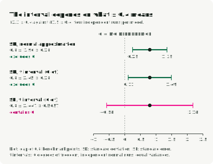
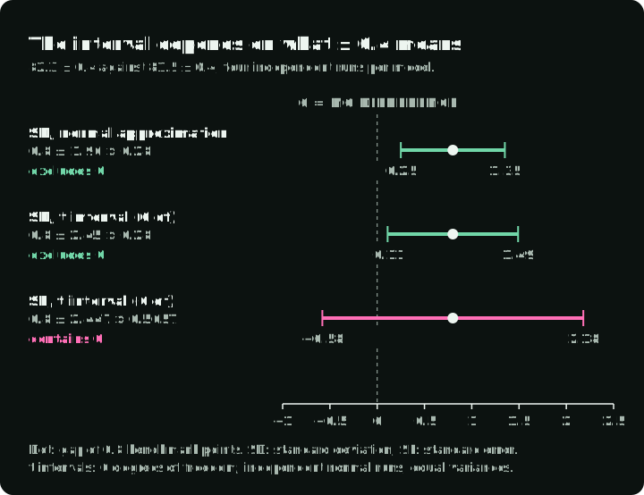
When 0.4 is the standard deviation, the t interval excludes zero: under these assumptions, the results support a positive difference. When 0.4 is the estimated standard error, the interval contains zero, so the results do not establish which model has the higher mean score.
Cross-entropy and KL divergence
During training, a model needs a numerical loss that measures how well its predicted probabilities agree with the training target. The training algorithm changes the model’s parameters to reduce that loss. Cross-entropy supplies such a loss for labeled examples or a teacher model’s probabilities. Kullback–Leibler (KL) divergence measures the mismatch between two distributions. Papers use it to train a student to imitate a teacher or to penalize changes from a fixed reference model.
Here the outcomes are discrete, such as tokens or classes. Write the target distribution as and the model’s predicted distribution over the same outcomes as . Start with one observed outcome : when the model gave it probability , its loss is . It is 0 when , about 0.69 when , about 2.3 when , and infinite when .
Cross-entropy averages that loss over outcomes drawn from the target:
With a one-hot label , which is 1 on the correct class and 0 elsewhere, only the correct class counts, and : the ordinary classification loss. PyTorch’s nn.CrossEntropyLoss computes this from raw model scores, called logits, and applies log-softmax internally; its input is not the probability vector . With a teacher model’s soft distribution as , every class counts in proportion to the teacher’s probability. Classical distillation trains a small model on a large model’s probabilities this way. For the target , two models have these cross-entropies :
The second model matches the target, and no model can do better. That minimum, 0.325 here, is , the entropy of . It is 0 only for a one-hot target: when the target itself is uncertain, some loss remains that no model can remove.
KL divergence subtracts that minimum and keeps only the loss caused by differing from . It is written with a double bar , which only separates the two arguments; it is neither the conditional-probability bar from Conditional probability and the probability of text nor the length bars of the vectors reference. Papers use it instead of a comma to mark that the order matters: the average runs over outcomes drawn from the first argument.
For the first model above, . KL is 0 when the two distributions match and positive otherwise.
The order changes which mismatches are penalized. A term with and is infinite, so penalizes for assigning zero probability to anything can produce. Outcomes with add nothing (by convention ), so they contribute no direct penalty even if . Reversing the arguments gives , which is infinite wherever and . Outcomes with now add nothing, even if . With as the target, is called the forward KL and the reverse KL.
For and , the forward KL is infinite, because misses an outcome produces, while the reverse KL is only : the outcome skips adds nothing. For and , the forward KL is the 0.37 found above, computed here term by term, and the reverse KL differs:
This asymmetry is why KL is called a divergence rather than a distance.
Because , and a fixed teacher’s entropy does not depend on the student, cross-entropy against a fixed teacher gives the student the same gradients as . Changing a student parameter changes both losses by the same amount, so their derivatives used for training are equal; Gradients and optimization explains that calculation. This lets classification and classical distillation code use cross-entropy. The swap works only with the teacher first. With the student first, , and the student’s own entropy changes as it trains, so the two no longer give the same gradients.
Vectors and matrices
Architecture equations describe calculations on arrays of numbers. An array’s shape tells you how its numbers are arranged, which operations are valid, and what those operations produce. A vector is an ordered list of numbers. A matrix arranges numbers in rows and columns. In ML code, tensor is the general term for these numerical arrays, including arrays with more than two axes. An axis is a dimension along which you index the array: a matrix has a row axis and a column axis.
A token’s hidden state is a vector of numbers computed inside the model to represent that token. Suppose we process a batch of sequences together, each with token positions, and each hidden state contains numbers. The hidden-state array has shape [B, T, d], which papers also write as . Its three axes select the sequence, the token position, and the number within that token’s vector. For example, [2, 3, 4] holds two sequences, three token vectors per sequence, and four numbers per vector: 24 numbers in total. Here is the vector’s width. The shape lists the three sizes; multiplying them gives the number of entries.
Papers often write shapes as set membership: means that is a vector of real numbers, and means that is a matrix with rows and columns. Bold letters sometimes mark vectors or tensors, but the paper’s definition determines the shape.
In the table below, and are column vectors: their numbers are arranged vertically. The superscript means transpose: exchange rows and columns. Thus is a row containing the same numbers as column . The capital and here name matrices; no longer means batch size.
| Expression | Values it uses | What the operation does | Result |
|---|---|---|---|
| — dot product | Two column vectors, each with entries | Multiply corresponding entries, then add the products: | One number |
| — outer product | A column with entries and a column with entries | Multiply every entry of by every entry of | An matrix; entry is |
| — matrix product | with rows and columns; with rows and columns | For entry , multiply corresponding numbers in row of and column of , then add | An matrix; ‘s column count must equal ‘s row count |
| — elementwise product | Two arrays of the same shape | Multiply entries at matching positions, without adding them | An array of the same shape |
| — concatenation | Columns and with and entries | Place the entries of after those of | One column with entries; check the paper’s convention for the joining axis |
For a concrete comparison, take and . Moving the transpose changes both the calculation and the result:
The dot product gives one score, as in the query–key comparison in attention. The outer product keeps a separate value for every pair of entries; the Gated DeltaNet update uses it to construct a matrix update from two vectors.
A matrix product can be regrouped, , but not reordered; the MLA derivation uses the regrouping to skip rebuilding keys. NumPy writes matrix multiplication as @ and the elementwise product as *. Papers do not inherit NumPy’s broadcasting rules: adding a vector to a matrix needs a stated axis. Papers also differ on whether a vector is a row or a column: attention stacks tokens as the rows of , while MLA, Gated DeltaNet and LoRA write with column vectors, and PyTorch’s nn.Linear computes x @ W.T on rows.
An architecture equation may also describe a vector’s size, restrict which matrices are allowed, or rearrange a product:
| Notation | Meaning |
|---|---|
| The Euclidean length; , without the root, appears in DDPM’s loss | |
| The sum of absolute values | |
| The spectral norm: the largest factor by which increases a vector’s length; mHC keeps it at most 1 | |
| The number of independent columns; LoRA’s update has rank at most | |
| The determinant: is the factor by which scales volume, and the sign records whether flips orientation; the change-of-variables example in this article’s Appendix B uses it | |
| Every entry is nonnegative, as in mHC; is a different condition, positive semidefinite: for every | |
| , | The identity matrix (1 on its diagonal, 0 elsewhere, so ); a vector of ones |
| Transposing a product reverses the order; Part 2’s RoPE and MLA sections use it |
Gradients and optimization
Training uses derivatives to decide how to change the model’s parameters. Let be one scalar loss and the vector of all parameters; is one entry in that vector.
The partial derivative is one number, evaluated at the current parameter values. It measures the loss’s rate of change when only changes and the other parameters stay fixed. Read it as “the partial derivative of the loss with respect to parameter ”.
The gradient collects those numbers for every parameter into one vector. Its th entry is . The symbol is called nabla; here it means “take the gradient”. With only one parameter, the gradient has one entry equal to the ordinary derivative.
For example, take . At and :
The first partial derivative, 4, means that increasing by 0.01 raises the loss by approximately 0.04 while stays fixed. The gradient contains this information for both parameters. Gradient descent subtracts each parameter’s derivative, multiplied by a positive learning rate that controls the step size:
With , the example changes from to , and the loss falls from 7 to 3.04. For a differentiable loss with a nonzero gradient, a sufficiently small step lowers the loss. A zero gradient gives no update.
The subscript on says what varies. varies the parameters; varies the input, and diffusion papers call it the score, which has nothing to do with a benchmark score.
A Jacobian records derivatives for several outputs. A neural-network layer can produce many numbers, such as the components of a token’s hidden state. To describe how every output responds to every input, collect the partial derivatives into a matrix called the Jacobian. For with input numbers and output numbers, its shape is : rows correspond to outputs, columns to inputs, and entry measures how output changes when input changes.
For example, let a function take two numbers and return and . Its Jacobian is
The second column says that increasing by 0.1 while holding fixed increases by 0.2 and decreases by 0.1. This example is linear, so its Jacobian is constant. For a nonlinear function, the entries can depend on the current input and describe small changes locally. With just one scalar output, the Jacobian has one row: the same derivatives as the gradient, transposed under our column-vector convention. Deep Learning, §4.3, gives the general definitions.
Backpropagation uses these derivatives to compute the loss gradient through successive layers. The change-of-variables example in this article’s Appendix B uses a different property: the absolute value of a square Jacobian’s determinant gives the local volume scaling factor, which is needed to adjust a probability density.
For training, derivatives describe local changes; an optimization objective states what the updates should minimize or maximize. Papers distinguish the best value of an objective from the parameters that achieve it: is the smallest value of , while gives the parameter values that achieve it. For , the minimum is 0 and the argmin is 3. An argmin specifies the desired result, but leaves the update algorithm open.
For example, MiniLLM writes its goal as (equation 1), where is the student model and the teacher it learns from. Section 2.2 then derives a gradient and modifies it to make training more stable; equation (7) is the gradient used for updates. The on-policy distillation example explains those changes. Reading only the argmin would miss them.
A stop-gradient, , passes forward unchanged but blocks gradients through it, like .detach() in PyTorch. Two expressions with the same forward value can train differently if one of them is detached. In the GRPO example, Hugging Face TRL treats the old model’s log-probability as fixed. In the distillation shortcut discussed by DeepSeek-V4, a detached teacher–student log-ratio supplies a fixed weight for the update.
Sets and constraints
A constraint states which values are allowed. Papers often express constraints using sets: collections of distinct members, written in braces, such as . Order does not matter, so names the same set. Repeated entries count only once. By comparison, the parentheses in a vector such as describe an ordered list: is a different vector.
Once a paper defines a set, it can test membership, combine sets, count their members or state a condition on them. Take and :
| Notation | Meaning | Example and how to read it |
|---|---|---|
| Membership: belongs to | : 2 is a member of | |
| Union: include every member of either set | ; include 3 only once | |
| Intersection: keep only members shared by both sets | ||
| The number of distinct members | ||
| ”For every”: a condition must hold for all the named members | : every member of is positive | |
| ”There exists”: at least one member must satisfy the condition | : has a member greater than 2, namely 3 |
The shape notation from Vectors and matrices also names sets: is the set of all vectors of real numbers, and the set of all real matrices with rows and columns. Thus specifies which shape must have.
Set-builder notation describes a set by a condition: reads “the members of that satisfy the condition”, like the Python set comprehension {x for x in S if condition(x)}. The bar means “such that”, not conditional probability; some papers use a colon instead. Examples in this series include mHC’s allowed matrices, MoE’s selected experts and sparse attention’s selected tokens.
DAPO, a training method that filters groups of generated answers, keeps a question only when some answers are correct and some are wrong. For sampled answers and reference answer , write the set of correct answer indices as
The filter is . Using indices makes the counting explicit: two samples with identical text still count as two answers. DAPO’s paper writes the set over the answers instead; read literally as a set of texts, that form counts two identical answers once.
Exercises
- Shapes. is , is and is . What are the shapes of the scores and of the output? Over which axis does softmax run?
- Softmax. Compute the softmax of . Does adding 100 to both inputs change the result?
- Averages. One answer has a single token with loss 4; another has three tokens with loss 0. Compute the per-token average and the per-answer average.
- Conditioning. Of 200 responses, 120 are correct, 80 pass format validation and 60 do both. Find and .
- KL. For a teacher and a student , compute both KL directions.
- Sets. DAPO keeps a question only if , where contains the indices of correct answers among samples. With , does it keep a question whose answers score ? One whose answers score ? Does the first answer change if all four samples contain identical correct text?
Answers:
-
The scores are and the output is . Softmax runs across the six keys in each query’s row.
-
. Adding the same number to every input leaves softmax unchanged, but computing directly overflows in 32-bit floats.
-
The two averages:
-
and .
-
, and , because the student puts probability on an outcome the teacher rules out.
-
No: has four members, which equals . Yes: has three members, between 0 and 4. Identical text does not change the first answer: these are four separate samples, so their four indices still count.
Appendix A. Greek letters
The roles are common examples; each paper still defines what its symbols mean.
| Letter | Name | Common roles in ML papers |
|---|---|---|
| alpha | A mixing weight or scale; a decay (Gated DeltaNet); a noise schedule (DDPM) | |
| beta | A penalty strength (DPO, GRPO); a writing strength (Gated DeltaNet); a noise schedule (DDPM) | |
| gamma | A discount factor in RL; a step size (the bias update in DeepSeek-V3) | |
| delta | A difference or a change | |
| epsilon | Noise (DDPM); a clipping range (GRPO); a small stabilizer | |
| eta | The learning rate | |
| theta | Model parameters; RoPE’s rotation angles | |
| lambda | A regularization weight; an eigenvalue | |
| mu | A mean; the number of gradient steps per batch in DeepSeekMath’s Algorithm 1 | |
| pi | A policy; is the product operator | |
| rho | A probability ratio, as in Part 3’s GRPO section; a correlation | |
| sigma | The sigmoid (DPO); a standard deviation; a covariance; is the sum operator | |
| tau | A temperature; a threshold; a trajectory in RL | |
| phi | The parameters of a second network, such as an encoder; features; an angle | |
| psi | The parameters of another network, such as the value model in DeepSeekMath’s PPO | |
| omega | A frequency; is also a lower bound in complexity, or a set of outcomes |
Variants such as and are usually the same letter in a different font, but a paper can use both for different variables.
Appendix B. Other equation families
Equation forms this series does not work through, with the definitions each needs:
Selective state-space models. A state-space model processes a sequence by updating a stored state at each step. An update of the form , combines the previous state with the current input, then computes an output. Here is the current input, the stored state and the output. The matrices , and respectively transform the previous state, add the input’s contribution and produce the output. The bars mark parameters converted from a continuous-time model to discrete steps; they do not mean averages. In Mamba, the update parameters depend on the current input, which is what “selective” means.
Stochastic differential equations. describes how a state changes with time : is its rate of change. A stochastic differential equation (SDE) adds random changes, . Here describes the deterministic change, sets the noise scale, and is an increment of Brownian motion. To approximate it in code, the Euler–Maruyama method uses a small time step and replaces with Gaussian noise of variance . Section 5.1 of Tianhua Chen’s The Little Book of Generative AI Foundations gives such an update; §6.4 of the same book uses SDEs to describe diffusion models.
Change of variables. Transforming a random variable changes its density according to how the transformation changes local volume. Suppose maps between spaces of the same dimension, and both and its inverse are differentiable. The densities before and after the transformation, and , satisfy . The inverse recovers from . Its Jacobian is the square matrix of first derivatives; the absolute value of its determinant corrects for the local change in volume. For example, if in one dimension, the density becomes : doubling the width halves the density. Normalizing flows use invertible transformations like this to model densities; Tianhua Chen’s book, §7.1, explains the method.
Min–max objectives. In generative adversarial networks (GANs), a generator produces examples and a discriminator tries to distinguish them from real data. The objective measures the discriminator’s success: maximizes it while minimizes it. The goal (equation 1) says: for each possible generator, consider the best discriminator against it, then choose the generator with the smallest resulting objective. Training does not solve that inner maximization exactly. The paper’s Algorithm 1 alternates gradient-ascent steps on with one gradient-descent step on ; its experiments used .
The probability simplex. A probability vector has nonnegative entries that add up to 1. The set of all such vectors with entries is called the probability simplex, written . Every softmax output lies in it. Here names a set, and the superscript is its dimension, not a power: once probabilities are chosen, the last must make the sum equal 1. With two choices, every distribution has the form for , so only one number is free.
Normalization. Normalization rescales values by the mean and spread of a chosen group. A common form is , where is a mean, a variance, and a small positive number that prevents division by zero. The equation alone does not say which entries are used to compute the mean and variance. For a batch of feature vectors, batch normalization computes them separately for each feature across examples. A Transformer’s layer normalization computes them separately for each token across its features. Check the specified axes when comparing implementations.
Sources and versions
Section and equation numbers refer to the versions linked here.
- Tianhua Chen. The Little Book of Generative AI Foundations: An Intuitive Mathematical Primer. 2026. Version 2; §2.4 and §3.2 cover Jensen’s inequality and the ELBO, §5.1 and §6.4 continuous-time noise.
- Vaswani et al. Attention Is All You Need. 2017. Version 7, §3.2.1, equation (1), and footnote 4.
- Dai et al. DeepSeekMoE: Towards Ultimate Expert Specialization in Mixture-of-Experts Language Models. 2024. Fine-grained expert segmentation and the combination counts, §3.1; ablation, §4.4 and Figure 3.
- Shao et al. DeepSeekMath: Pushing the Limits of Mathematical Reasoning in Open Language Models. 2024. Version 3, §1.1, §4.1.1, equations (1)–(4), and Algorithm 1.
- DeepSeek-AI. DeepSeek-V2: A Strong, Economical, and Efficient Mixture-of-Experts Language Model. 2024. Version 5, §2.1.1–2.1.3, equations (9)–(19), and Appendix C.
- DeepSeek-AI. DeepSeek-V3 Technical Report. 2024–2025. Version 2, §2.1.2, equations (12)–(18).
- DeepSeek-AI. DeepSeek-R1: Incentivizing Reasoning Capability in LLMs via Reinforcement Learning. 2025. Version 1: §2.2.1, equations (1)–(3). Version 2, 2026: §2.1 and Supplementary A.3.
- DeepSeek-AI. DeepSeek-V4: Towards Highly Efficient Million-Token Context Intelligence. 2026. Version 1: §2.2, equations (1)–(8); §5.1.2, equation (29).
- Rafailov et al. Direct Preference Optimization: Your Language Model is Secretly a Reward Model. 2023–2024. Version 3, §4, equation (7).
- Gu et al. MiniLLM: Knowledge Distillation of Large Language Models. 2023–2024. Version 4, §2.1, equation (1), and §2.2, equations (2) and (7).
- Yu et al. DAPO: An Open-Source LLM Reinforcement Learning System at Scale. 2025. Version 2, §3.2–3.3, equations (11)–(12).
- Gu and Dao. Mamba: Linear-Time Sequence Modeling with Selective State Spaces. 2023–2024.
- Yang et al. Gated Delta Networks: Improving Mamba2 with Delta Rule. 2024–2025. Version 3, §3.1, equation (10), and §3.3–3.4.
- Ho, Jain and Abbeel. Denoising Diffusion Probabilistic Models. 2020. Version 2, §2, equations (4)–(5); §3.2, equation (12); §3.4, equation (14); and Algorithms 1–2.
- Goodfellow et al. Generative Adversarial Nets. 2014. Equation (1) and Algorithm 1.
- Chen et al. Evaluating Large Language Models Trained on Code. 2021. Version 2, §2.1, equation (1), and Figure 3.
- Hugging Face TRL.
GRPOTrainerandGRPOConfigat commitc6eac19, October 2026. - Stanford CS229. Probability Theory Review and Linear Algebra Review and Reference.
- Dive into Deep Learning. Preliminaries.
- Britz, Goldie, Luong and Le. Massive Exploration of Neural Machine Translation Architectures. 2017. Version 2, Table 5; cited by Attention Is All You Need for dot-product against additive attention.