RAG Evaluation Metrics: Retrieval, Reranking, Generation

For engineers operating or evaluating retrieval-augmented generation (RAG) systems, this reference maps failures in document parsing, filtering, retrieval, reranking, and generation to the metric that identifies each one. It also shows which checks run before release and which monitor live traffic.
A RAG system with broken relevance filters can run for months without triggering an operational alert. It still returns answers and meets its latency target, but the answers rely on incomplete evidence. Recall@k against the original eligible gold set exposes the loss. Latency and availability dashboards do not.
Want to skip ahead and run code?
The runnable
slavadubrov/rag-evals-demorepository separates SciFact retrieval, generation on labeled synthetic QA, and offline fixture checks.make evalruns retrieval, filter diagnostics, and generation fixture replay aftermake index.make benchmarksweeps chunking and embedding settings without API calls; the comparison of two OpenAI models needs an API key and the--liveflag (see Part 8). Notebooks 00–09 cover retrieval, filtering, generation, and system examples. The demo uses embedded Qdrant, so it does not require Docker.
RAG evaluation decision table
Use this table as the starting point before choosing a framework. The right metric depends on the failure mode you are trying to catch, not on the tool name.
| Question | Metric family | Use this when | Watch out for |
|---|---|---|---|
| Did parsing preserve the source? | Extraction completeness, table/figure coverage | PDFs, slides, scans, and HTML pages enter the corpus | Clean-looking text can still drop captions, footnotes, or table structure |
| Did retrieval find the right evidence? | Recall@k, nDCG@k, MRR, context precision/recall | You can label relevant chunks or documents | A hard metadata filter can remove the correct document before ranking starts |
| Did reranking improve the shortlist? | Reranker uplift, Precision@1, nDCG delta | Cross-encoders or LLM rankers sit after retrieval | Measure latency and cost with the quality gain |
| Did the answer use the evidence? | Faithfulness, groundedness, citation support | The answer cites documents or claims facts from context | Faithfulness cannot diagnose bad parsing or bad retrieval |
| Is the system stable in production? | Drift, regeneration, fallback, p95 latency, cost per answer | Traffic changes after launch | Production telemetry needs sampled human review to stay calibrated |
For a shorter tool comparison, see Best RAG Evaluation Tools: Ragas, DeepEval, and TruLens.
Part 1: Define success before the architecture
Draft the eval set before the architecture diagram. It gives each later component choice a measurable target.
You cannot choose between BM25 and dense retrieval, recursive and semantic chunking, or Cohere Rerank and BGE until you know what you are optimizing. “Better answers” is not a metric. An illustrative release requirement is “faithfulness ≥ 0.85 on a 200-query golden set covering our top three intents, with p95 latency < 1.5s and filter false-exclusion rate < 2%.” Its numbers are placeholders; the important part is that quality, coverage, latency, and filtering have explicit thresholds.
Define the harness before you write the retrieval code. The first harness will be wrong, and you will revise it. Revising a metric is much cheaper than revising a system you have already shipped.
Three pipeline layers and two run modes
Production evaluation has three pipeline layers. Ingestion evaluation asks whether the corpus and index preserve the source. Query-time evaluation asks whether rewriting, filtering, retrieval, reranking, and context assembly found the right evidence. Answer and production evaluation asks whether the response used that evidence and whether quality holds under live traffic. Collapse the layers into one score and a normalization bug can disappear inside an acceptable answer score.
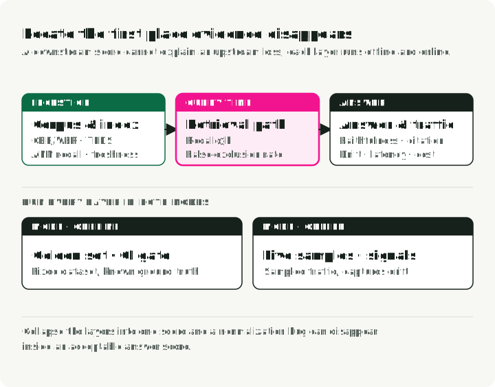
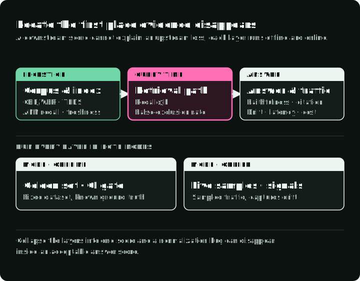
Those layers describe where a failure happens. Offline and online describe when and against which data the check runs. Offline evaluation uses a fixed dataset with known ground truth; it is reproducible and belongs in component selection, A/B comparisons, and CI checks that can block a change. Online evaluation scores sampled live traffic and captures regeneration, dwell time, explicit feedback, and real query drift. It is noisier and harder to instrument.
Use both modes where they help: fixed corpora and query sets make regressions reproducible; sampled live traces expose freshness failures and drift.
Component-level vs. end-to-end
There are two common mistakes. End-to-end-only evaluation tells you the system is broken, but not where. Component-only evaluation can show every part passing while the full system still fails. The fix is a few headline end-to-end metrics for go/no-go decisions, plus component metrics for diagnosis. Retrieval metrics catch retriever regressions. Generation metrics catch generator regressions. End-to-end answer correctness catches integration failures.
The reference frameworks (opinionated tour)
| Framework | Best at | Where it falls down |
|---|---|---|
| RAGAS | A shared vocabulary for faithfulness, answer relevancy, and context precision/recall (metrics) | LLM-judge cost; opaque score components when debugging; version changes |
| ARES | A task-specific classifier judge, if training and annotation are worth the cost (paper); its reported precision is benchmark-bound | Heavier setup; you have to actually train models |
| TruLens | Trace-linked feedback functions and OpenTelemetry integration (project) | Less batteries-included on RAG-specific metrics than RAGAS |
| DeepEval | Test-runner integration and custom metrics (project) | Heavy LLM-judge usage = cost spikes |
| Arize Phoenix | Tracing, dataset experiments, and prebuilt or custom RAG/agent evaluators (evaluation docs) | Domain rubrics and judge thresholds still need local calibration |
| TREC 2024 RAG Track | Public benchmark for nugget evaluation (AutoNuggetizer), support evaluation, and fluency on MS MARCO Segment v2.1 | Not a runtime tool; a benchmark to calibrate against |
My default stack is RAGAS for the metric vocabulary, DeepEval for CI checks, Phoenix for production tracing, plus custom code for ontology-specific metrics. Pick the framework that makes custom metrics easy.
For benchmark selection, match the task before reading the leaderboard. BEIR, MTEB, and MIRACL remain useful retrieval baselines. Add tests for capabilities they do not establish:
- Current end-to-end RAG: the TREC 2026 RAG Track uses narrative queries and ClimbMix-400b, replacing MS MARCO v2.1, and links the RAGDoll evaluation toolkit. Its 2026 topics are released; judgments are not yet published. Use the topics for experiments, not as a judged leaderboard. Keep the 2024 and 2025 protocols below tied to their own corpora and judgments.
- Technical questions against evolving code: FreshStack combines human-asked Stack Overflow questions, repository corpora, and nugget judgments. Its released snapshot and its machinery for building new corpora are different things; pin the repository revision and question date.
- Images that carry part of the question or evidence: MM-BRIGHT separates text-to-text, multimodal-to-text, multimodal-to-image, and multimodal-to-multimodal retrieval. Score the relevant task separately. OCR text alone may omit what a chart or screenshot contributes.
These benchmarks extend coverage; they do not replace the eligible, versioned query set from your application.
Part 2: Map evaluation points
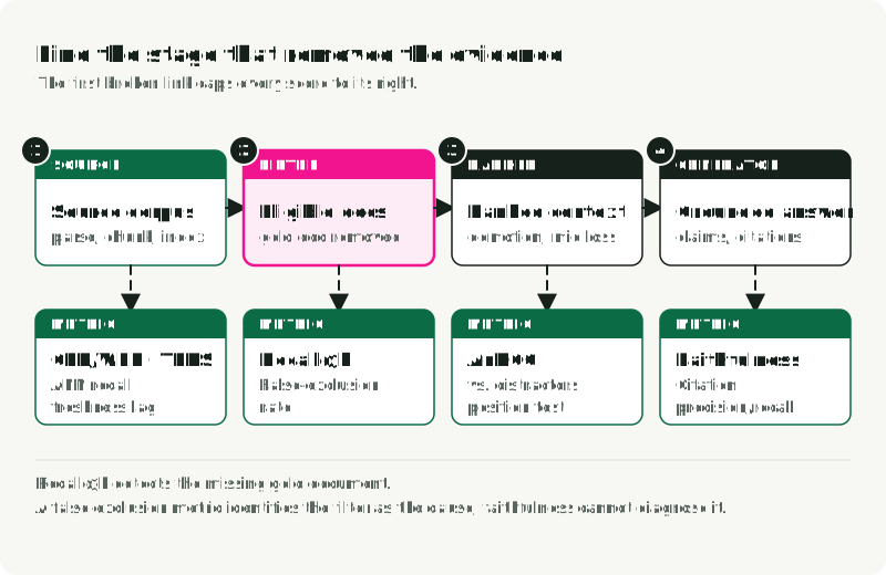
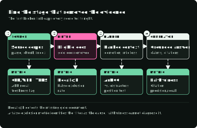
When an answer is wrong or unsupported, follow the gold document through the four checks in the figure, left to right. The first stage where it is missing names the metric to check first and the part of this article that covers it.
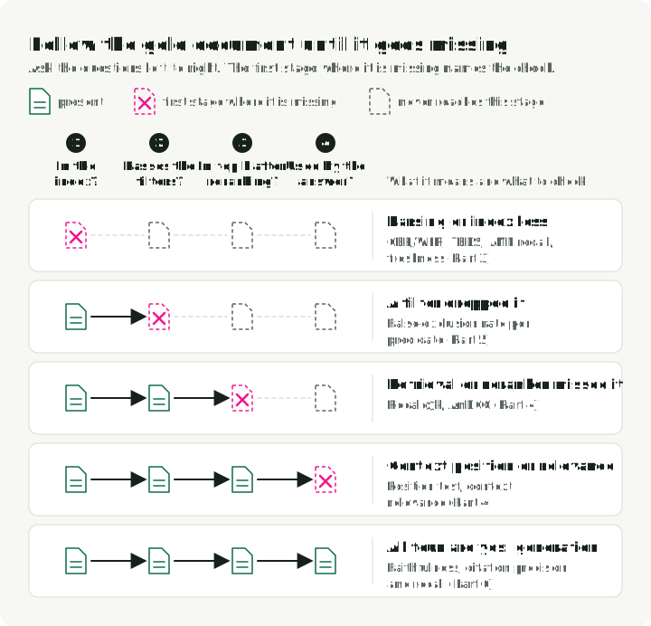
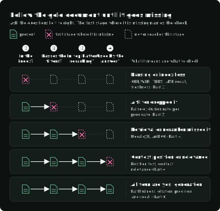
Upstream losses cap downstream quality: bad parsing caps retrieval, and bad retrieval caps reranking and generation. Faithfulness measures the answer, never the upstream cause.
Part 3: Ingestion evaluation
Many production RAG failures start in ingestion. The system works on clean test documents, then fails on real PDFs, scans, tables, and messy corpus pages.
Document acquisition and parsing
What to measure:
-
Extraction length sanity check:
extracted_chars / expected_charsper document class flags suspicious length changes, but duplicated or wrong text can still score 1.0. Compare aligned text against a hand-cleaned reference for omissions and substitutions, then check footnotes, captions, table content, and reading order separately. -
OCR accuracy: CER (Character Error Rate) and WER (Word Error Rate), the standard speech/OCR metrics:
where , , are character-level substitutions, deletions, insertions and is the reference character count (subscript for the word version). Do not apply one CER boundary to every corpus. Calibrate it by document class and downstream answer loss. Printed text, handwriting, and multilingual material have different error profiles. Compute with
jiwer(jiwer.cer(refs, hyps),jiwer.wer(refs, hyps)) or HuggingFaceevaluate. For evaluation corpora, FUNSD and SROIE are public benchmarks.from jiwer import cer, wer refs = ["Mars has two moons, Phobos and Deimos."] hyps = ["Mars has two m00ns, Phobos and Deirnos."] print(f"CER = {cer(refs, hyps):.3f}") # CER = 0.105 print(f"WER = {wer(refs, hyps):.3f}") # WER = 0.286 -
Table extraction fidelity: TEDS (Tree-Edit-Distance-based Similarity) measures how close a predicted HTML table tree is to the reference, normalized by the size of the larger tree. From Zhong et al., 2020 (PubTabNet):
TEDS uses both structure (rows, columns, spans) and cell content. TEDS-S strips the content and scores structure only. Reference implementation: PubTabNet’s
src/metric.py(usesaptedunder the hood). For evaluation corpora, see PubTabNet, FinTabNet, and SciTSR. Naive parsers often fail on tables. Benchmark before trusting them. -
Layout / structure preservation: heading order, list integrity, reading order on multi-column PDFs. Use DocLayNet for a labeled benchmark. An off-the-shelf comparison can span an element parser such as
unstructured, a PDF library such aspymupdf, and a selected Docling pipeline. Docling offers standard and VLM paths; record which one you test.
Compare distinct parser families, for example a Tesseract baseline, a VLM-based OCR model, and your vendor candidate. Best OCR models compares the current options. Use a stratified sample of real document classes at a fixed DPI, including clean scans, photos, tables, multilingual text, math, and handwriting. Report CER or WER for each class and TEDS for table pages.
Cleaning and normalization
-
Boilerplate removal accuracy: precision/recall against human-labeled boilerplate spans. Aggressive removal drops relevant content; lazy removal pollutes embeddings. Tools to compare:
trafilatura,jusText,Resiliparse. Barbaresi (2021) compares Trafilatura with baselines including jusText; Resiliparse is a separate candidate, not a system evaluated in that paper. -
Unicode normalization: percent of documents producing identical NFC and NFKC outputs (computed with the stdlib
unicodedata.normalize) is a useful compatibility-form drift signal. It does not detect invisible/default-ignorable code points or cross-script lookalikes: scan for the former explicitly and apply a Unicode confusables policy or detector when the latter is in scope. -
Language detection accuracy: F1 on a labeled multilingual sample. Critical for multilingual indexes. Use
fasttext-langdetect(Facebook’slid.176),lingua-py, orcld3. FLORES-200 supplies evaluation text across 200 languages, but your production language mix should determine the test slice. -
Deduplication effectiveness (MinHash / LSH): precision/recall of your near-duplicate detector against a hand-labeled set. The underlying idea: estimate Jaccard similarity between document shingle sets via random permutation hashes (Broder, 1997) and bucket near-duplicates with LSH banding (Indyk & Motwani, 1998). Sweep the hash count and Jaccard threshold on your corpus. Track false-merge rate (corrupts answers) separately from missed-merge rate (wastes index space).
datasketchprovides the implementation used below; its parameters are illustrative:from datasketch import MinHash, MinHashLSH def shingles(text: str, k: int = 5) -> set[str]: text = text.lower() return {text[i:i + k] for i in range(len(text) - k + 1)} def to_minhash(text: str, num_perm: int = 128) -> MinHash: m = MinHash(num_perm=num_perm) for s in shingles(text): m.update(s.encode("utf-8")) return m docs = { "d1": "Mars has two moons, Phobos and Deimos.", "d2": "Mars has two moons, Phobos and Deimos!", # near-dup "d3": "Curiosity rover landed on Mars in 2012.", } lsh = MinHashLSH(threshold=0.8, num_perm=128) for did, text in docs.items(): lsh.insert(did, to_minhash(text)) print(sorted(lsh.query(to_minhash(docs["d1"])))) # ['d1', 'd2'] -
PII scrubbing: precision and recall, computed separately per entity type (emails, SSNs, names, addresses). Recall errors create compliance risk; precision errors hurt answer quality. Set the operating point with the legal team. Candidate tools include Microsoft Presidio,
scrubadub, or a fine-tuned NER model on a labeled set.
Chunking controls retrieval quality
Chunking changes which evidence reaches the answer. In NVIDIA’s 2025 vendor benchmark, page-level chunking achieved the highest average end-to-end answer accuracy in the tested setup, which preserved tables and charts as whole units. That measures answer accuracy, not retrieval recall. Treat that result as evidence for the tested corpus rather than a universal winner.
Semantic chunking groups adjacent sentences by embedding similarity and cuts at dissimilar boundaries. LangChain’s SemanticChunker and LlamaIndex’s SemanticSplitterNodeParser implement this strategy. It can improve recall over fixed windows when topical boundaries matter.
LangChain’s RecursiveCharacterTextSplitter tries double newlines, single newlines, spaces, then individual characters by default: ["\n\n", "\n", " ", ""]. It does not detect sentence boundaries unless you configure suitable separators or use a sentence-aware splitter. Its default length_function=len measures characters. To try 400–512 tokens per chunk with 10–20% overlap, use a token-counting length function. Treat these as starting settings and compare them with other values on your golden set.
Metrics to track:
- Chunk coherence: , where are sentence embeddings. Healthy chunks are internally similar and at-boundary dissimilar. Compute with
sentence-transformersplusscikit-learn’scosine_similarity. - Boundary quality: human-labeled “is this a sensible cut?” on a sample, plus a structural check that chunks don’t split tables, lists, or numbered sections.
- Optimal chunk size: sweep token sizes (128, 256, 512, 1024) and plot Recall@k vs. size on your golden set. Pick the smallest size after which Recall@k stops improving.
- Overlap effectiveness: sweep overlap at 0, 10, 20, and 30% as a starting grid and measure Recall@k. Stop increasing overlap when the local recall curve flattens or duplication cost outweighs the gain.
- Chunk attribution fidelity: percent of chunks that retain a verifiable source pointer (page number, section anchor, doc ID). Auditability requires this.
- Late vs. early chunking: late chunking (Günther et al., 2024) embeds the full document then segments, preserving global context (reference implementation in
jina-embeddings-v3). Contextual Retrieval (Anthropic, 2024) prepends LLM-generated context to each chunk. Both add cost. Benchmark on your corpus before adopting either one.
My opinion: structural chunking (splitting on headings, tables, and sections — implemented by parsers like unstructured.io or by walking the AST your parser already produced) is underused. If your documents have structure, use it before adding similarity heuristics. Recursive character splitting is the baseline; semantic chunking is worth the overhead mainly on unstructured prose.
Metadata extraction and enrichment
- NER precision/recall/F1: per entity type, on a labeled subset. Standard CoNLL/MUC-style. Compute with
seqeval(from seqeval.metrics import f1_score) for the BIO/IOB-tag-aware version, or scikit-learn for span-set comparisons. CoNLL-2003 and OntoNotes 5.0 are the canonical reference corpora. - Relation extraction F1: even more important for ontology-grounded systems. Hand-label a set stratified by relation type and document class. TACRED and DocRED are public benchmarks; candidate implementations include
opennreandspaCyrelation pipelines. - Title / heading extraction accuracy: exact-match plus normalized Levenshtein similarity () against ground truth —
python-Levenshteinorrapidfuzzgive you both in one call. - Hierarchical metadata preservation: percent of chunks that correctly retain their parent section, parent document, and ancestry path. This is the metric that decides whether your RAG can answer “what does the child of policy X say?” type questions.
Embedding generation
- Model selection benchmarks: Use MTEB’s retrieval-task results, BEIR for zero-shot generalization, and MIRACL for multilingual retrieval as comparison points. MTEB retrieval commonly reports nDCG@10; other task families use other metrics. The MTEB Python package runs the benchmarks locally. Treat transfer from English MTEB to a lower-resource language as a hypothesis to test on that language’s labeled set.
- Domain-specific evaluation: do not treat a general benchmark rank as a domain result. Start with a few hundred labeled queries (200–500) across your main query types; Part 9 shows how to check whether that is enough. Then re-rank candidate models on it with
ranxorpytrec_eval. A domain set can reverse a leaderboard ordering, so publish the dataset slice, retrieval protocol, and confidence interval with the result. - Embedding drift detection: compare two collections of embeddings: a fixed reference sample and a rolling current sample. Maximum mean discrepancy (MMD) tests whether their distributions differ. Another option is a validated classifier trained to distinguish reference from current samples. Kullback–Leibler (KL) divergence compares probability distributions, so it needs an explicit estimator, such as chosen histograms; raw embedding coordinates are not probabilities. Also measure nearest-neighbor stability for a fixed probe set.
evidentlyandalibi-detectimplement model-based and statistical detectors. Evidently’s comparative study is one vendor evaluation; compare methods on known shifts in your own embeddings. - Multi-vector vs. single-vector: late interaction preserves token-level representations instead of collapsing each document into one vector; ColBERT is the canonical design, with reference implementations in RAGatouille and PyLate. That richer representation increases index and retrieval cost. Compare quality, storage, and latency against a single-vector baseline on the same domain set before adopting it.
Index construction
- Recall@k under approximation: compare the approximate-nearest-neighbour (ANN) index against an exact brute-force baseline at the same k — in FAISS, that’s
IndexHNSWFlat(orIndexIVFFlat) vs.IndexFlatIP/IndexFlatL2. As a first check, require Recall@10 of at least 0.95 against exact search, then tighten or relax it from your downstream answer quality. Theann-benchmarksproject tracks recall–QPS Pareto curves across libraries. - HNSW tuning: HNSW (Hierarchical Navigable Small World) is a layered proximity graph; see Malkov & Yashunin, 2018. It is implemented in
hnswlib, FAISS’sIndexHNSWFlat, and most vector DBs. HNSW exposes three knobs:M(graph fan-out),efConstruction(build-time candidate width), andefSearch(query-time candidate width). Starting values:Mof 16–32 andefConstructionof 100–200; then raiseefSearchuntil Recall@10 against exact search stops improving. The hnswlib parameter guide saysMof 12–48 suits most uses and gives a check forefConstruction: withefset toefConstruction, recall forMnearest neighbors below 0.9 means the graph can still improve. - IVF tuning: IVF (Inverted File index — partition vectors with k-means into
nlistcells, then at query time scan thenprobenearest cells; see FAISS’sIndexIVFFlatandIndexIVFPQ). The FAISS index guidelines suggest 4√N to 16√N cells for N vectors as a startingnlist. Sweepnlistandnprobeagainst exact-search recall and latency. Benchmark filtered queries separately because index families and vector databases implement filter traversal differently. - Update freshness lag: time from doc commit to retrievability. Track p50 and p99. For systems with regulatory requirements, also track the percent of queries served against stale indexes.
Part 4: Query-time evaluation
The query-time lane contains the metrics that diagnose a retrieval path. Recall@k alone cannot show whether rewriting, filtering, reranking, or context assembly caused the failure.
Query understanding and rewriting
- Query expansion quality: Recall@k uplift on your golden set, expanded query vs. raw. Predefine the minimum useful gain and its uncertainty before testing. If expansion does not meet that requirement, it does not justify its latency and cost. Classical PRF (pseudo-relevance feedback) baselines like RM3 and Bo1 are still useful sanity checks; LLM-based expansion needs to beat them.
- HyDE evaluation: HyDE (Gao et al., 2022) generates a hypothetical answer with the LLM, embeds it, and retrieves against that. It adds a generation call, and that call can invent content that pulls retrieval off topic. Measure Recall@10 separately on in-domain, out-of-domain, and low-confidence slices, then choose whether it belongs in the default path, a fallback, or neither.
- Multi-query generation: Recall@k union of N rewrites vs. single query. Sweep N and choose a point on your recall–latency frontier. Implementations: LangChain’s
MultiQueryRetriever, LlamaIndex’sQueryFusionRetriever. - Intent classification accuracy: standard precision/recall/F1 per intent (compute with
sklearn.metrics.classification_report), but the operative metric is routing correctness — does the right downstream pipeline get invoked? - Adaptive routing: Adaptive-RAG (Jeong et al., NAACL 2024) makes the case that not every query deserves the same retrieval strategy. Track router accuracy as a classification problem against a labeled set of “needs no retrieval / one-shot / iterative.”
Iterative search needs a budgeted end-to-end test
An agent can search, inspect a result, and search again instead of retrieving one fixed top-k list. The banking_knowledge domain in tau2-bench switches retrieval with a --retrieval-config flag: no knowledge base, the full knowledge base in context, BM25 or embedding search, a sandboxed shell tool, or BM25, dense search, and the shell together. For a local comparison, give one-shot and iterative retrieval the same eligible corpus and explicit limits on time, model tokens, and tool calls. Record each query and evidence seen at each turn; score final evidence coverage, answer correctness, citation support, and exhausted-budget failures. More search calls are useful only when the added evidence improves the answer within those limits.
The companion’s retrieval/iterative.py runs supplied query reformulations under explicit call, time, and token budgets. For agents that choose their own searches, AI agent evaluation: traces to test suites covers how to score the trajectory as well as the answer.
Retrieval metrics
These are the baseline metrics. If you do not track them, you cannot tell whether retrieval is improving.
| Metric | What it measures | When to use |
|---|---|---|
| Recall@k | fraction of a query’s relevant documents returned in top k | use when missing any part of the relevant set matters |
| Precision@k | percent of top-k that are relevant | useful when context window is the bottleneck |
| MRR | average of 1/rank of the first relevant doc | when users only look at the top-1 or top-3 |
| nDCG@k | position-discounted gain weighted by relevance grades | standard retrieval metric for graded relevance |
| MAP | mean over queries of average precision | when you care about the entire ranked list |
| Hit Rate@k | whether at least one relevant document appears in top k | average the binary result across queries for a quick sanity metric |
| Coverage | percent of golden docs ever retrieved across all queries | catches systematic gaps in the index |
The formulas, for reference (binary relevance with relevant set for query , and if the -th retrieved doc is in ):
For graded relevance, ; binary nDCG is the special case used in the code below. MAP is the mean over queries of . See Manning, Raghavan, Schütze, Introduction to Information Retrieval, chapter 8 for derivations.
For production code, use ranx, pytrec_eval, or ir_measures — they implement the entire TREC metric family and handle graded relevance correctly. As starting release gates, the companion repo ships Recall@10 ≥ 0.85 and MRR ≥ 0.6 (in .env.example, applied with --quality-gates). Then tune them on your golden set against downstream answer quality and the cost of a miss.
Here, k counts unique document IDs. Reject duplicates rather than giving a repeated document extra gain. For chunking experiments, declare whether k counts chunks or deduplicated parent documents, and also compare evidence supplied within a fixed token budget. The same document recall can hide very different context quality.
The test harness for these is short. You can run it from a notebook before you’ve even chosen a vector database.
from math import log2
from statistics import mean

# synthetic gold set: query_id -> set of relevant doc ids
gold = {
    "q1": {"d3"},
    "q2": {"d7", "d2"},
    "q3": {"d11"},
    "q4": {"d5"},
}

# ranked retrieval results: query_id -> ranked list of doc ids (top-10)
runs = {
    "q1": ["d8", "d3", "d1", "d4", "d2", "d9", "d6", "d10", "d12", "d13"],
    "q2": ["d2", "d6", "d4", "d7", "d1", "d3", "d8", "d11", "d5", "d9"],
    "q3": ["d11", "d2", "d3", "d4", "d1", "d6", "d7", "d8", "d10", "d12"],
    "q4": ["d1", "d2", "d3", "d6", "d8", "d9", "d10", "d12", "d13", "d14"],
}

def recall_at_k(ranked, gold_set, k):
    if k <= 0 or len(ranked) != len(set(ranked)):
        raise ValueError("require positive k and unique document IDs")
    if not gold_set:
        return 0.0
    hit = sum(1 for d in ranked[:k] if d in gold_set)
    return hit / len(gold_set)

def reciprocal_rank(ranked, gold_set):
    if len(ranked) != len(set(ranked)):
        raise ValueError("require unique document IDs")
    # MRR contribution per query: 1/rank of the first relevant doc.
    for rank, d in enumerate(ranked, start=1):
        if d in gold_set:
            return 1.0 / rank
    return 0.0

def ndcg_at_k(ranked, gold_set, k):
    if k <= 0 or len(ranked) != len(set(ranked)):
        raise ValueError("require positive k and unique document IDs")
    # binary relevance: rel ∈ {0, 1}
    gains = [1.0 if d in gold_set else 0.0 for d in ranked[:k]]
    dcg = sum(g / log2(i + 2) for i, g in enumerate(gains))
    # ideal DCG: all gold docs ranked first, capped by k
    n_gold_in_topk = min(k, len(gold_set))
    idcg = sum(1.0 / log2(i + 2) for i in range(n_gold_in_topk))
    return dcg / idcg if idcg else 0.0

K = 5
print(f"Recall@{K}: {mean(recall_at_k(runs.get(q, []), gold[q], K) for q in gold):.3f}")
print(f"MRR:       {mean(reciprocal_rank(runs.get(q, []), gold[q]) for q in gold):.3f}")
print(f"nDCG@{K}:  {mean(ndcg_at_k(runs.get(q, []), gold[q], K) for q in gold):.3f}")
# Recall@5: 0.750
# MRR:       0.625
# nDCG@5:    0.627
# Duplicate and missing runs are tested in the companion's tests/test_audit_contracts.py.
The aggregate iterates over all expected queries, treating a missing run as empty. This example assigns zero to empty-gold queries; in a real suite, mark those as a separate answerability slice with its own denominator rather than treating the zero as measured recall. Report timeouts and missing runs as well as scores.
Run a fast subset on every PR and the full golden set before release (Part 9 gives starting sizes). Block a merge when a metric you chose in advance crosses its regression budget.
The companion repo pins the exact numbers above (Recall@5 = 0.750, MRR = 0.625, nDCG@5 = 0.627) as a unit test in tests/test_retrieval_metrics.py. Notebook 01 runs this k=5 example, then reports Recall@10, MRR, and nDCG@10 on a SciFact slice; it does not sweep k. The production-shaped harness lives in evaluation/retrieval.py.
Hybrid retrieval and reciprocal rank fusion
BM25 is a sparse lexical scorer that combines exact-term matching, term weighting, and length normalization. It is available in rank_bm25, Elasticsearch, OpenSearch, and most search engines.
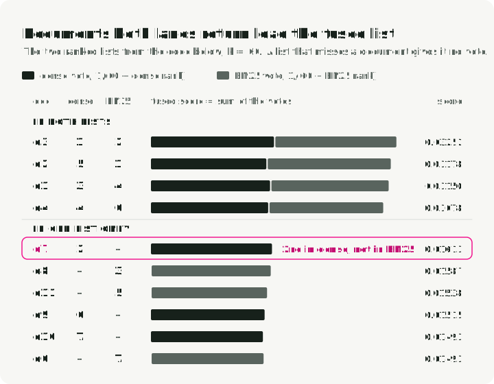
Reciprocal Rank Fusion (Cormack, Clarke, and Buettcher, SIGIR 2009) combines BM25 and dense rankings by position. The original k=60 setting is a useful baseline. RRF is score-agnostic, which avoids the cross-lane normalization required by linear interpolation. With a labeled set large enough to estimate a stable delta, also test a convex combination and tune α.
My hypothesis is that hybrid retrieval plus a cross-encoder reranker can help technical, log-style, and code corpora. The gain may be small on heavily semantic corpora. Measure against the dense-only and sparse-only lanes because a poor fusion configuration can underperform either input. The companion SciFact notebook is one bounded test, not a general result.
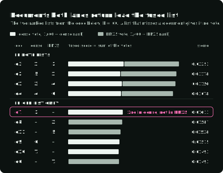
The chart uses the two ranked lists from the code below. Each lane adds 1/(60 + rank) for every document it returns, so the four documents in both lists lead. d7 ranks second in the dense list but is not in the BM25 list, so it falls to fifth.
The implementation fits in a few lines.
from collections import defaultdict

# two retrieval lanes: dense embeddings and BM25.
dense  = ["d3", "d7", "d1", "d4", "d2", "d9", "d10"]
sparse = ["d2", "d3", "d8", "d1", "d11", "d4", "d6"]

def rrf(rankings: list[list[str]], k: int = 60) -> list[tuple[str, float]]:
    """Reciprocal Rank Fusion (Cormack et al., SIGIR 2009).

    score(d) = sum over rankings of 1 / (k + rank(d))
    Score-agnostic: only rank position matters. k=60 is the canonical default.
    """
    scores: dict[str, float] = defaultdict(float)
    if k <= 0:
        raise ValueError("k must be positive")
    for ranking in rankings:
        if len(ranking) != len(set(ranking)):
            raise ValueError("each ranking must contain unique document IDs")
        for rank, doc in enumerate(ranking, start=1):
            scores[doc] += 1.0 / (k + rank)
    return sorted(scores.items(), key=lambda kv: kv[1], reverse=True)

fused = rrf([dense, sparse], k=60)
for doc, score in fused[:5]:
    print(f"{doc}  score={score:.5f}")
# d3  score=0.03252   <- rank 1 dense, rank 2 sparse
# d2  score=0.03178   <- rank 5 dense, rank 1 sparse
# d1  score=0.03150
assert [doc for doc, _ in fused[:3]] == ["d3", "d2", "d1"]
Note what RRF doesn’t do: it never looks at the raw similarity scores. If a retriever puts a document at position 2, that vote is worth 1 / (60 + 2), whatever raw score produced it. A dense retriever returning cosine 0.98 and a BM25 lane returning score 17.4 are not directly comparable. Z-score and min-max normalization remove affine scale differences, but neither calibrates a score as relevance. Outliers, distribution shape, and the candidate set still affect the normalized values and therefore the fusion result. Validate any score-based combination on labeled queries.
Hybrid + RRF on SciFact: notebook 02 compares dense vs BM25 vs RRF using aggregate Recall@10, MRR, and nDCG@10. The production-shaped fuser is in retrieval/hybrid_rrf.py; tests/test_rrf.py pins the canonical d3 / d2 / d1 ordering at k=60.
Reranking
- ΔnDCG / ΔMRR: uplift over no-rerank, on your golden set, at the depth your application actually uses. Compute by running your retrieval metrics with and without the reranker on identical candidate sets.
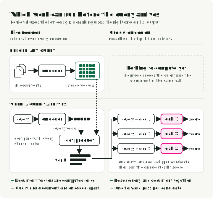
- Cross-encoder vs. bi-encoder: a bi-encoder embeds query and doc independently (one vector per side) and scores by dot product; a cross-encoder concatenates query+doc and runs a single forward pass that attends jointly across both. Cross-encoders trade a forward pass per candidate for richer query–document interaction; the figure below shows the difference. Reference implementation:
sentence-transformersCrossEncoder. Benchmark relevance and latency on named hardware, batch size, and candidate depth; do not transfer one model or managed service’s result into another environment. - Listwise vs. pointwise: pointwise scores each (query, doc) pair independently; listwise scores the whole candidate list jointly so the model can compare candidates. Evaluate both on the same candidate sets. Calibrate any score threshold per model and corpus rather than treating a published example as portable.
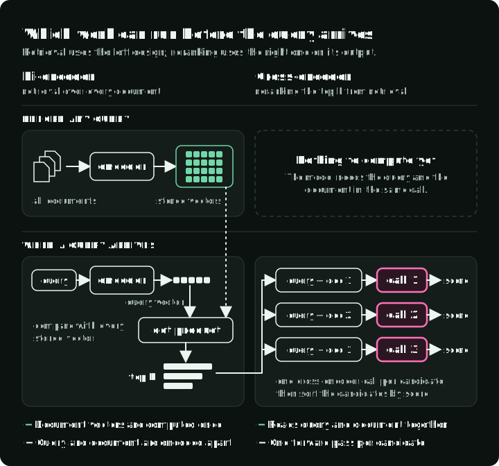
In the figure, compare the two time bands. The bi-encoder encodes every document before any query and stores the vectors; when a query arrives, it encodes only the query. The cross-encoder has nothing to compute before the query. It reads query and document in one model call, so it runs once per candidate and only on the short list that retrieval returns.
The code below scores three candidates for one query with a BGE cross-encoder:
from sentence_transformers import CrossEncoder

reranker = CrossEncoder("BAAI/bge-reranker-v2-m3")  # Reproducible baseline, not a latest-model ranking

query = "How do I rotate database credentials in production?"
candidates = [
    "Production database credentials are rotated via Vault every 30 days.",
    "The new logo was unveiled at the all-hands meeting.",
    "To rotate prod DB creds, run the `rotate-secrets` GitHub Action.",
]

scores = reranker.predict([(query, c) for c in candidates])
ranked = sorted(zip(candidates, scores), key=lambda x: -x[1])
for doc, score in ranked:
    print(f"{score:+.3f}  {doc}")
The BGE code above is a small baseline. For a current comparison, include Cohere Rerank 4.0 fast/pro for managed multilingual text ranking, or Qwen3-VL-Reranker 2B/8B when queries or documents include images, screenshots, or video. Keep task modalities, candidate depth, input limits, instructions, and hardware explicit.
A reranker often helps a basic RAG pipeline, but it is not a guaranteed win. Measure its ΔPrecision@1 and ΔnDCG on your golden set, then keep it only if the gain clears its latency and cost budget. Compare that measured gain with smaller retrieval changes before choosing the next optimization. BM25 vs embeddings vs rerankers gives a shorter guide to choosing each layer of the ranking stack.
Notebook 03 reports P@10 before and after cross-encoder reranking on SciFact, plus ΔnDCG@10; module: retrieval/reranker.py. The evaluation/reranking.py module compares rerankers on identical candidate pools.
Context construction and lost-in-the-middle
Many “good retrieval, bad answer” failures start in context construction.
- Context relevance: Ragas
ContextRelevancejudges the supplied context list using two prompts and normalized ratings; it is not a per-chunk score. For chunk diagnostics, score each query–chunk pair explicitly, for example with a cross-encoder, and report the distribution under a locally calibrated threshold. - Supplied-context citation coverage: distinct supplied chunks cited divided by distinct chunks supplied. Report empty-context cases separately. This observable proxy says which chunks received citations, not which ones the model internally used or whether the citations support its claims. Check citation support separately and compare coverage with answer quality and token cost.
- Lost-in-the-middle detection: synthetic eval where you place the gold chunk at positions {first, middle, last} of a long context and measure answer correctness. The cited Liu et al. (TACL 2024) study reports U-shaped degradation under its long-context conditions. Treat the same pattern in a current model as a hypothesis to test. Mitigations: rerank then reorder the top-k so the highest-scored chunk is first or last (LangChain’s
LongContextReorderdoes exactly this), or compress middle chunks aggressively. Measure with a position-stratified eval, not just an aggregate score. A worked, runnable position-stratified eval lives in notebook 06 (module:evaluation/lost_in_middle.py). - Context compression: report compression ratio (input tokens / output tokens) alongside answer correctness. Tools include LangChain’s
ContextualCompressionRetrieverand LongLLMLingua. Predefine the largest acceptable correctness loss from the application’s risk and token budget, then reject configurations that cross it.
Part 5: The filter false-exclusion rate
This metric gets its own section because aggregate retrieval scores cannot attribute a miss to a relevance filter. Evaluate eligibility filters separately against caller entitlements; a document outside that set must remain excluded.
A hard relevance predicate such as product = Y AND locale = en-US can drop effective recall to zero among documents the caller is allowed to see. Correctly implemented Recall@k catches the loss because its denominator remains the original eligible relevant-document set. It does not tell you whether the filter, retriever, or ranker caused the miss. Faithfulness judges claims against the retrieved context. It may still score claims supported by that incomplete context, but it cannot diagnose the filter or retrieval cause. An empty refusal may produce no statements and NaN, depending on the implementation; do not treat it as evidence that faithfulness approved the refusal.
The diagram runs the worked example below. The entitlement check removes d3, which belongs to another tenant; that exclusion is correct. The relevance filter then removes the gold document for q1 and q3. Recall@10 falls to 50% and registers the drop; only the false-exclusion rate, also 50%, attributes it to the predicate. An evaluator that rebuilds the gold set after filtering reports 100%.
The metric
filter_false_exclusion_rate =
    (# queries where all gold docs were excluded by metadata filter) /
    (# queries with at least one entitlement-eligible gold doc)
This query-level definition counts catastrophic exclusions: no eligible relevant document survives. Intersect each query’s gold set with the caller’s entitlement set before scoring; an ineligible document is not a false exclusion. For multi-gold queries, standard Recall@k still exposes partial loss; add a per-document exclusion rate if that boundary matters. To compute either rate, you need (a) ground-truth doc IDs for each eval query and (b) instrumentation that logs the filter predicates applied, not just the final results. As a starting gate, the companion uses a false-exclusion rate of at most 2%; tune it from the cost of excluding a valid answer and the confidence interval of your production sample.
Here’s a working implementation. It compares correct standard recall with an invalid evaluator that redefines relevance after filtering.
# A small worked example where relevance predicates remove eligible documents.
docs = [
    {"id": "d1", "tenant": "acme",   "locale": "en-US"},
    {"id": "d2", "tenant": "acme",   "locale": "en-GB"},
    {"id": "d3", "tenant": "globex", "locale": "en-US"},
    {"id": "d4", "tenant": "acme",   "locale": "en-US"},
    {"id": "d5", "tenant": "acme",   "locale": "de-DE"},
    {"id": "d6", "tenant": "acme",   "locale": "fr-FR"},
]

# Tenant isolation is an eligibility invariant, not a relevance experiment.
# Verify it independently before evaluating relevance preferences.
eligible_docs = [d for d in docs if d["tenant"] == "acme"]
assert {d["id"] for d in eligible_docs} == {"d1", "d2", "d4", "d5", "d6"}

queries = [
    # the gold doc lives in en-GB but the dynamic filter forced en-US
    {"qid": "q1", "gold": {"d2"}, "filter": lambda d: d["locale"] == "en-US"},
    # the gold doc is correctly within the tenant filter
    {"qid": "q2", "gold": {"d4"}, "filter": lambda d: d["tenant"] == "acme"},
    # the gold doc lives in fr-FR but the dynamic filter forced en-US
    {"qid": "q3", "gold": {"d6"}, "filter": lambda d: d["locale"] == "en-US"},
    # the gold doc passes the filter (de-DE locale match)
    {"qid": "q4", "gold": {"d5"}, "filter": lambda d: d["locale"] == "de-DE"},
]

def filter_false_exclusion_rate(queries, eligible_docs):
    n_with_gold, n_excluded = 0, 0
    eligible_ids = {d["id"] for d in eligible_docs}
    for q in queries:
        eligible_gold = q["gold"] & eligible_ids
        if not eligible_gold:
            continue
        n_with_gold += 1
        survivors = {d["id"] for d in eligible_docs if q["filter"](d)}
        if not (eligible_gold & survivors):
            n_excluded += 1
    if not n_with_gold:
        raise ValueError("false-exclusion rate needs queries with eligible gold")
    return n_excluded / n_with_gold, n_with_gold

rate, eligible_query_count = filter_false_exclusion_rate(queries, eligible_docs)
print(f"filter_false_exclusion_rate = {rate:.2%}")
# filter_false_exclusion_rate = 50.00%
print(f"eligible queries = {eligible_query_count} / {len(queries)}")
# eligible queries = 4 / 4

# Correct Recall@k keeps the original eligible gold set as its denominator.
def standard_recall_at_k(queries, eligible_docs, k=10):
    recalls = []
    eligible_ids = {d["id"] for d in eligible_docs}
    for q in queries:
        eligible_gold = q["gold"] & eligible_ids
        if not eligible_gold:
            continue
        # demo only: the survivor set stands in for a ranked run.
        # A real harness ranks the survivors first, then slices to k.
        survivors = [d for d in eligible_docs if q["filter"](d)][:k]
        survivor_ids = {d["id"] for d in survivors}
        recalls.append(len(eligible_gold & survivor_ids) / len(eligible_gold))
    return sum(recalls) / len(recalls) if recalls else 0.0

print(f"standard recall@10 = {standard_recall_at_k(queries, eligible_docs):.2%}")
# standard recall@10 = 50.00%

# INVALID: rebuilding the gold set after filtering changes the question.
# It drops queries whose relevant documents did not survive, then scores 100%.
def invalid_recall_over_filtered_gold(queries, eligible_docs, k=10):
    recalls = []
    all_doc_ids = {d["id"] for d in eligible_docs}
    for q in queries:
        all_survivors = {d["id"] for d in eligible_docs if q["filter"](d)}
        filtered_gold = q["gold"] & all_doc_ids & all_survivors
        if not filtered_gold:
            continue
        top_k_ids = set(list(all_survivors)[:k])
        recalls.append(len(filtered_gold & top_k_ids) / len(filtered_gold))
    return sum(recalls) / len(recalls) if recalls else 0.0

invalid = invalid_recall_over_filtered_gold(queries, eligible_docs)
print(f"INVALID recall (filtered gold) = {invalid:.2%}")
# INVALID recall (filtered gold) = 100.00%

assert rate == 0.5
assert standard_recall_at_k(queries, eligible_docs) == 0.5
assert invalid == 1.0
# Unauthorized gold and an empty denominator are tested in the companion's
# tests/test_audit_contracts.py.
The function returns the rate and the number of queries with eligible gold. If that denominator is empty, it raises instead of reporting a reassuring zero; a required release check must treat that as missing evidence. Queries with only unauthorized gold remain in separate entitlement tests.
Half the queries lose their gold doc to the filter, so correct Recall@10 falls to 50%. That score catches the symptom but cannot attribute it. The false-exclusion rate shows that the predicate removed two answers before the retriever ran. The deliberately invalid evaluator reports 100% only because it discards those failures from its gold set. No model can recover a document that was filtered out.
The companion’s tests/test_filter_exclusion.py::test_50_percent_exclusion_rate and the first example in notebook 04 use an older five-document fixture that also scores 50%, but its q3 is excluded by tenant isolation. That fixture does not reproduce the eligible-gold example above. Notebook 04 also runs SciFact filter diagnostics with synthetic metadata. The current evaluation/filter_exclusion.py accepts a separate authorization predicate and a fixed eligible-gold set, and includes predicate precision/recall.
Companion metric: predicate precision and recall
When filtering is dynamic (for example, an LLM extracts filter predicates from the query), treat the predicate extractor as a classification model and evaluate it as one. Measure predicate precision and recall against a labeled set of (query, correct predicate) pairs. A predicate error rate does not map directly to the same point loss in retrieval recall; measure how often those errors exclude a gold document. Once a hard filter removes the gold document, no amount of reranking helps.
Eligibility filters vs. relevance preferences
Authorization, tenant isolation, legal jurisdiction, and publication state determine whether a document may enter the candidate set. Keep them as hard filters and validate them independently; Recall@k, false-exclusion rate, and relevance precision do not authorize their relaxation.
For a relevance preference such as locale, recency, or version, compare a hard predicate with a soft boost on the same held-out, eligible queries. Two rules decide the outcome:
- Access rules (authorization, tenant, jurisdiction, publication status) are always hard filters.
- Any other preference is a soft boost, unless the measured test below passes. Then it may become a hard predicate.
The pseudo-code gives the test for rule 2:
For each relevance preference F:
  hard_recall_F  = retrieval_recall@k with F as a hard filter
  soft_recall_F  = retrieval_recall@k with F as a +0.X rerank boost
  hard_precision = relevant_in_top_k / k under hard filter
  soft_precision = relevant_in_top_k / k under soft boost
  precision_gain = hard_precision - soft_precision
  precision_gain_CI = paired-query uncertainty interval for precision_gain
  exclusion_rate = % of queries where the gold doc was filtered out (hard)

Pre-register Δ_min, ε, and recall_loss_max for this workflow.
Use a hard predicate only if:
  lower_bound(precision_gain_CI) >= Δ_min
  AND exclusion_rate <= ε
  AND hard_recall - soft_recall >= -recall_loss_max.
Otherwise prefer a soft boost.
Choose the minimum useful precision gain, uncertainty interval, ε, and recall-loss bound from the harm of excluding an otherwise eligible answer, the benefit of added precision, and the size of the held-out sample. Start with an ε of 1–2%, and lower it where a missed answer is costly.
Part 6: Generation evaluation
Retrieval metrics tell you the system could answer correctly. They do not tell you it did. Generation metrics cover that gap.
Faithfulness and groundedness
RAGAS faithfulness decomposes the answer into atomic claims (short, self-contained factual statements), then verifies each against the retrieved context via an LLM judge:
Faithfulness checks support in the supplied evidence; it does not establish that the evidence is correct or sufficient to answer the question. Record no-claim responses separately and report their count rather than assigning perfect faithfulness to an empty answer.
The current Ragas documentation recommends the collections API below. In a uv project, install ragas and openai with uv add ragas openai, set OPENAI_API_KEY, and save this as a script to run with uv run. It makes provider calls and incurs their charges; the score is a judge result, not a deterministic expected constant. Pin the resolved dependencies in your lockfile.
import asyncio

from openai import AsyncOpenAI, omit
from ragas.llms import llm_factory
from ragas.metrics.collections import Faithfulness

async def main():
    async with AsyncOpenAI() as client:
        # Ragas 0.4.3 sends max_tokens by default; GPT-5.6 models need max_completion_tokens.
        llm = llm_factory(
            "gpt-5.6-terra", client=client, reasoning_effort="none",
            max_tokens=omit, max_completion_tokens=1024,
            temperature=omit, top_p=omit,
        )
        scorer = Faithfulness(llm=llm)
        result = await scorer.ascore(
            user_input="How many moons does Mars have?",
            response="Mars has two moons, Phobos and Deimos.",
            retrieved_contexts=["Mars has two moons named Phobos and Deimos."],
        )
        print(result.value)

if __name__ == "__main__":
    asyncio.run(main())
This example uses GPT-5.6 Terra as the judge; the Ragas factory forwards model arguments. Compare the judge’s false passes, false failures, and cost against human labels before you replace a cheaper judge that you have already checked against labels.
The framework table in Part 1 also names answer relevancy and context precision. The same collections API scores both with the same llm. AnswerRelevancy also takes an embedding model, for example embedding_factory("openai", model="text-embedding-3-small", client=client) from ragas.embeddings.base. ContextPrecision needs a reference answer in ascore. Each score answers a different question: faithfulness asks whether the context supports the answer, answer relevancy asks whether the answer addresses the question, and context precision asks whether the relevant context ranks first.
To build your own scorer, keep the extract–verify–aggregate structure. Extraction is an LLM call that splits the answer into claims; verification is an NLI (natural-language inference) model or an LLM judge. Validate extraction and entailment separately, and record no-claim or failed judgments. For example, an answer with 4 claims, 3 of them supported, scores 3/4 = 0.75. An answer with 0 claims is not scored.
Notebook 05 runs a fixed Mars example offline with a lexical proxy; that proxy does not verify semantic entailment. Its module, evaluation/faithfulness.py, also implements SGR claim extraction and verification. The generation suite evaluates labeled synthetic QA with --suite generation --live. The companion uses OpenAI models only. gpt-5.6-luna generates and judges by default; --judge-model gpt-5.6-terra changes the judge. Both models come from one provider, so the repo shows the judge workflow, not a cross-family comparison.
A purpose-built alternative to LLM-as-judge is HHEM-2.1-Open (Hughes Hallucination Evaluation Model, Vectara), a classifier fine-tuned for hallucination detection. Its model card documents the checkpoint, the raw 0–1 score it emits, and balanced-accuracy results on AggreFact and RAGTruth. It publishes no default decision boundary, so picking one is your job. Treat those as model-card evidence, not a guarantee on your corpus: calibrate the threshold on local labels and compare it with your chosen judge before deployment.
Atomic-fact evaluation
FActScore (Min et al., EMNLP 2023) decomposes long-form generations into atomic facts, retrieves evidence per fact, labels each supported / not-supported, and reports the supported fraction:
Reference implementation: shmsw25/FActScore. The original evaluation focused on biographies with Wikipedia as evidence. Adaptations to summaries or other long-form domains need local verification of claim extraction, evidence coverage, and support judgments. Watch out: repetitive trivial facts can inflate the score, and individually true statements can form a misleading answer. MontageLie (EMNLP 2025) tests this weakness through deceptive relationships and ordering among true statements. VeriScore handles claims with necessary modifiers; the Core filter helps prevent fact-padding.
Citation accuracy
Track citation precision (cited spans actually support the claim) and citation recall (claims that should be cited, are):
The TREC 2024 RAG Track defines a reproducible support evaluation protocol. Thakur et al. (SIGIR 2025) report roughly 56% agreement with human judgments made from scratch and 72% under a different condition where humans post-edited LLM predictions. The latter is assisted annotation, not independent evidence of a judge accuracy improvement. Keep the annotation condition attached to the number. For an automated approximation, ALCE (Gao et al., EMNLP 2023) implements citation precision/recall with NLI-based verification.
Answer correctness, completeness, refusal
- Answer correctness against a reference: exact match or token-F1 can suit short answers; Hugging Face
evaluate.load("squad")computes both, and thebert-scorepackage computes BERTScore. For longer answers, check factual relations, entities, quantities, negation, and required information against reviewed references. BERTScore and embedding cosine measure similarity; a wrong number or negation can preserve a high score. RagasAnswerCorrectnesscombines factual comparison with similarity rather than equating the two. - Completeness via nuggets: a nugget is a relevant information unit, with vital nuggets distinguished from optional useful ones. A founding-date question may require the year; the founder’s name is not automatically required. AutoNuggetizer constructs and refines nuggets from judged document pools, then checks their presence in generated answers. Its initial TREC 2024 report covered 21 topics and 45 runs. The TREC 2025 overview, published March 2026, extends the protocol to narrative queries and evaluates retrieval relevance, answer completeness, and attribution. These are public evaluation protocols, not evidence that every production RAG system needs the same nugget rubric.
- Refusal behavior: label whether the supplied evidence permits an answer, then measure correct refusals among all refusals and refusals among cases that should abstain. NoMIRACL (Findings of EMNLP 2024) tests robustness against relevant and non-relevant supplied passages; it does not prove the entire corpus has no answer. Separate retrieval misses from genuinely out-of-scope queries in your own suite.
Post-generation verification
The cheapest reliability gains often come from deterministic post-checks, not larger models.
-
Unseen-entity flag: record named-entity strings in the answer that are absent from a normalized context string (for example,
spaCy’sentsplus exact matching). This is a cheap, domain-specific flag for unseen entity strings, not a grounding check: it cannot establish identity, relation, negation, time, or provenance. Measure its precision and recall on local labels before using it to approve a release, and retain claim-level entailment or human review for verification.In this example the flag finds no unseen entity, although the answer says the opposite of the context.
def unseen_entity_flag(answer: str, context: str, entities: list[str]) -> bool: return any(entity.lower() not in context.lower() for entity in entities) context = "Paris was not founded in 1994." answer = "Paris was founded in 1994." assert not unseen_entity_flag(answer, context, ["Paris"]) claim_supported = False # human label or an NLI verdict, not the lexical flag assert not claim_supported -
Claim verification: extract claims, run NLI against context, fail or flag any below threshold. NLI-as-faithfulness models:
cross-encoder/nli-deberta-v3-large,MoritzLaurer/DeBERTa-v3-large-mnli-fever-anli-ling-wanli. Adds latency. Worth it for high-stakes domains. -
Self-consistency (Wang et al., ICLR 2023): sample multiple generations at temperature > 0; report agreement rate (e.g., proportion of generations that match the modal answer, or pairwise BERTScore); choose the sample count from the stability–cost curve and flag low-agreement answers for human review.
-
Confidence calibration: collect verbalized confidence (“How confident are you, 0–1?”) and compare to actual correctness on the eval set. Plot a calibration curve and report Expected Calibration Error: , where are confidence bins. Implementations:
netcal,torchmetrics.CalibrationError. A model that reports 0.9 confidence should be correct on roughly 90% of comparable cases; measure the gap instead of assuming calibration.
Part 7: Ontology-grounded RAG evaluation
The standard metrics above cover open-corpus RAG. If your RAG retrieves against a structured ontology, taxonomy, or knowledge graph, those metrics are necessary but not sufficient. Examples include products in a catalog, conditions in SNOMED, components in a BOM, and security techniques in MITRE ATT&CK. You also need to measure the ontology layer.
Entity linking accuracy
The first task is mapping a query mention to an ontology entity (“Aspirin” → wikidata:Q18216, “the 737” → aircraft:Boeing_737).
- Mention-level precision/recall/F1: standard, against gold mention spans (compute with
seqevalor a span-set comparator). - Disambiguation accuracy: of correctly-detected mentions, what fraction map to the right entity ID? Public references include ReFinED, REL, and GENRE; benchmarks like AIDA-CoNLL and BELB show that results vary by system and domain.
- NIL handling: precision/recall on “entity not in ontology.” Measure over-linking to near-but-wrong entities separately from correct abstention.
Hierarchy-aware evaluation
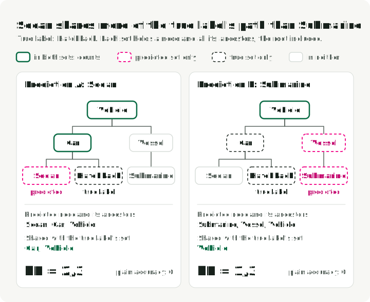
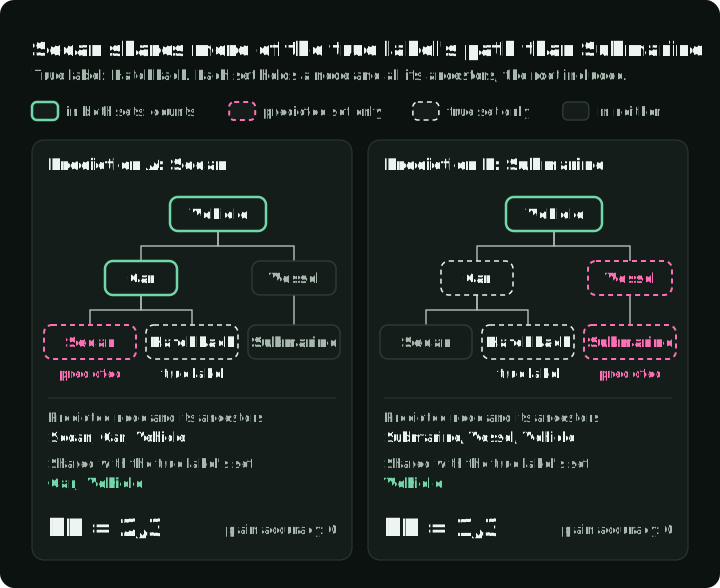
Plain accuracy treats “predicted Sedan when truth is Hatchback” the same as “predicted Submarine when truth is Hatchback.” Those errors are not equal. In the diagram, Sedan shares two of its three nodes with the true label, and Submarine shares only the root; the hierarchical precision below turns that overlap into a score.
-
Hierarchical precision/recall/F1 (Kosmopoulos et al., 2015): credit shared ancestors in the ontology DAG. With the predicted node plus all its ancestors and the true node plus all its ancestors:
Implement with
networkxon the ontology graph: augment each prediction and each label with its ancestors, then take the set overlaps above. -
Wu-Palmer similarity between predicted and gold entity in the taxonomy (Wu & Palmer, 1994):
where LCA is the lowest common ancestor in the taxonomy. Available out of the box in NLTK for WordNet (
from nltk.corpus import wordnet as wn; wn.synset("car.n.01").wup_similarity(wn.synset("truck.n.01"))); for custom taxonomies, compute LCA withnetworkx. -
Sibling/parent confusion rate: separately track confusions to siblings, parents, and children —
count_sibling / total_errors,count_parent / total_errors,count_descendant / total_errors. Use reviewed examples to test whether sibling errors come from ambiguous mentions or parent errors from over-generalization.
Filter false-exclusion rate (reprise, now critical)
In ontology-grounded systems, hard filters often come from the ontology itself (“only retrieve docs tagged with category X”). The exclusion-rate metric (defined in Part 5) becomes a primary correctness signal. A wrong category prediction can zero out recall; the exclusion rate attributes that loss to the filter.
Constrained generation conformance
When your output must conform to an ontology (every entity name in the answer must be a valid ontology member; every predicate must come from a closed vocabulary), measure:
- Schema validity rate: percent of outputs that parse and validate against the ontology schema. Validate with
jsonschemaorpydantic. JSONSchemaBench is the public benchmark for general structured output; for ontology-specific schemas, build your own validator. - Vocabulary conformance: percent of named entities in the output that are valid ontology IDs — a one-line set-membership check against the closed vocabulary.
- Semantic conformance: a syntactically valid output can still pick the wrong-but-valid entity. Pair conformance with downstream answer correctness.
Constrained decoding frameworks (Outlines, XGrammar, Guidance, OpenAI Structured Outputs) are designed to enforce schema validity. JSONSchemaBench compares efficiency, coverage, and quality across implementations. Re-run its cases that match your schemas and serving backend because coverage and latency depend on both.
Auditability
For ontology-grounded systems where answers face review:
- Citation completeness: percent of factual claims with at least one verifiable citation.
- Provenance depth: percent of citations that resolve all the way back to a source document with a stable ID, not just a chunk hash.
- Reproducibility rate: re-running the same query at a fixed snapshot returns the same answer. Pin the model version, runtime, decoding configuration, and seed, then set the required repeat rate from the workflow’s auditability needs. Temperature zero alone does not guarantee determinism. A miss can come from generation, the serving runtime, or any upstream stage.
Part 8: System-level evaluation
Holistic answer quality
- LLM-as-judge (Zheng et al., NeurIPS 2023): a scalable model-based evaluation approach. G-Eval (Liu et al., EMNLP 2023) generates evaluation steps from the task and criteria, then weights rating levels by their token probabilities: . These are probabilities, not log probabilities. Agreement depends on the judge, task, prompt, and calibration set.
- Pairwise preference: present judge with answer A vs. answer B; record preference. This replaces an absolute rating with a comparative decision, but still needs calibration against human preferences. MT-Bench reported GPT-4 judge agreement above 80% with both human preferences and human–human agreement under its benchmark conditions; do not transfer that rate to another domain without calibration.
LLM-as-judge has real biases:
- Position bias: measure order sensitivity on human-labeled cases for the selected judge and task. Randomization or swapped-order aggregation can help some model/task pairs, but retain either only when it improves local human agreement; the 2026 controlled study found position swapping harmful on its adversarial cases.
- Verbosity bias: judges can confound length with quality. The cited 2026 controlled study, version 2 found heterogeneous expansion-pair behavior: three judges preferred longer answers, Claude preferred concise answers, and GPT-4o was approximately neutral. All five performed well on truncation controls. Those results are benchmark-bound, so tell your judge how to treat completeness and filler, then report length-controlled performance on your own rubric.
- Self-preference risk: Zheng et al. observed a 10% higher GPT-4 self-win rate and a 25% higher Claude-v1 self-win rate in their data, but concluded that limited data and small differences could not establish self-enhancement bias. Compare same- and cross-family judges against local human labels; choose the better-calibrated judge rather than assuming either arrangement is safe.
Practical recipe: select a judge on human-labeled calibration data, mask model identities, measure order sensitivity, and state the length policy in the rubric. Repeat cases only when the added samples materially reduce uncertainty. For high-stakes evaluations, compare same- and cross-family judges and analyze disagreements against human labels.
Schema-Guided Reasoning for judges
Free-form output is one source of variation in judge runs. Two runs against the same answer may organize the rubric differently and produce different scores. Schema-Guided Reasoning (SGR) makes that rubric explicit: define the evaluation stages as a Pydantic schema, then use constrained output through Outlines, XGrammar, vLLM structured outputs, or OpenAI response_format to enforce the supported schema constraints. Field order may help a reviewer inspect the record, but it does not prove that the model reasoned through the stages in that order.
For RAG eval the schema decomposes the judgment into explicit, auditable fields rather than letting the model jump straight to a number:
from pydantic import BaseModel, Field, ValidationError, model_validator
from typing import Literal

class FaithfulnessJudgment(BaseModel):
    extracted_claims: list[str] = Field(
        description="Atomic factual claims in the answer, one per item."
    )
    supported_claims: list[str] = Field(
        description="Subset of extracted_claims that are entailed by the context."
    )
    unsupported_claims: list[str] = Field(
        description="Subset that is NOT entailed by the context."
    )
    outcome: Literal["scored", "no_claims"]
    failure_mode: Literal[
        "none", "fabrication", "overgeneralization", "wrong_entity", "stale_fact"
    ]
    rationale: str

    @model_validator(mode="after")
    def require_claim_partition(self):
        for claims in (self.extracted_claims, self.supported_claims, self.unsupported_claims):
            if any(not claim.strip() for claim in claims):
                raise ValueError("claims must contain non-whitespace text")
        extracted = set(self.extracted_claims)
        supported = set(self.supported_claims)
        unsupported = set(self.unsupported_claims)
        if not extracted:
            if supported or unsupported or self.outcome != "no_claims":
                raise ValueError("an empty extraction must be a no_claims outcome")
            return self
        if (
            len(extracted) != len(self.extracted_claims)
            or len(supported) != len(self.supported_claims)
            or len(unsupported) != len(self.unsupported_claims)
            or supported & unsupported
            or supported | unsupported != extracted
            or self.outcome != "scored"
        ):
            raise ValueError("verdict lists must be a complete, disjoint claim partition")
        return self

    @property
    def score(self) -> float | None:
        if not self.extracted_claims:
            return None
        return len(self.supported_claims) / len(self.extracted_claims)

valid = FaithfulnessJudgment(
    extracted_claims=["Mars has two moons", "Mars has a thick atmosphere"],
    supported_claims=["Mars has two moons"],
    unsupported_claims=["Mars has a thick atmosphere"],
    outcome="scored",
    failure_mode="fabrication",
    rationale="The atmosphere claim lacks support.",
)
assert valid.score == 0.5
empty = FaithfulnessJudgment(
    extracted_claims=[],
    supported_claims=[],
    unsupported_claims=[],
    outcome="no_claims",
    failure_mode="none",
    rationale="Score refusal correctness separately.",
)
assert empty.score is None
try:
    FaithfulnessJudgment(
        extracted_claims=["Mars has two moons"],
        supported_claims=["Mars has two moons"],
        unsupported_claims=["Mars has two moons"],
        outcome="scored",
        failure_mode="none",
        rationale="Contradictory verdict.",
    )
except ValidationError:
    pass
else:
    raise AssertionError("overlapping verdicts must fail validation")
This illustrative contract computes the score only after the verdict lists form a complete, disjoint partition of extracted claims. A no-claim outcome has no faithfulness score and must stay out of the faithfulness aggregate; report its count and score refusal correctness separately so abstentions cannot silently improve the average. Preserve those semantic checks in production; constrained output guarantees the shape, not an unbiased verdict. The Pydantic model also makes a rubric change visible as a code diff, while human calibration tests the judgment itself.
This works for any rubric-based judge, not just faithfulness. Pairwise preference, citation support, and refusal correctness all benefit from the same treatment.
Notebook 07 measures position bias with mirrored pairwise calls. Its module, evaluation/llm_judge.py, also implements pointwise SGR scoring. Pairwise runs present both answer orders and report swap consistency. The companion’s pointwise judge returns one integer score; it is not the probability-weighted G-Eval method. Because both companion models come from one provider, measuring self-preference still needs a cross-family judge compared against local human labels.
Latency and cost
- p50, p95, p99 at every pipeline stage. A reasonable start is p95 for the SLO and p99 for alerting; change either once you know the user journey, traffic volume, and error budget.
- Time-to-first-token vs. total generation time. Users care about TTFT for streaming UX.
- Stage breakdown: retrieval, reranking, generation, post-processing. Use the trace to locate the tail instead of assuming which stage caused it; record reranker device and batch size when comparing runs.
- Total $/query = embedding + retrieval + rerank + generation + storage amortized. Track p50 and p99; the long tail is where the budget goes.
- Cache hit rates at the embedding cache, retrieval cache, and KV-cache levels. Set separate targets from observed repetition, invalidation policy, and the cost avoided at each layer.
Notebook 08 displays p50/p95/p99 for the retrieve stage instrumented by evaluation/runner.py. The evaluation/latency.py module can summarize other stages when you instrument them explicitly. make benchmark sweeps chunking and embedding settings without API calls. The LLM comparison needs an OpenAI key and uv run python -m rag_evals.scripts.benchmark --skip-chunking --skip-embedding --live.
A/B testing
- Unit of randomization: first define the outcome you want to estimate. Then ask whether earlier answers can change later behavior, and whether one user’s assigned version can affect another user’s experience. Use per-user or per-session assignment when repeated exposure can change behavior or create inconsistent UX. Per-query assignment is defensible only when those effects are negligible and the analysis models repeated observations.
- Primary, guardrails, exploratory metrics: pre-register them. Choose the primary measure from the product outcome; satisfaction proxies include thumbs, regenerations, and dwell. Treat latency and cost as guardrails when they constrain the experience.
- Sample size: power-analyze before launching from the minimum effect worth detecting, baseline variance, assignment unit, and stopping rule.
Part 9: Test set construction
A metric is only as good as the test set it runs on. If your golden set covers three intents and production traffic spans twelve, Recall@10 measures only those three intents. Worse, a test set that overfits to easy questions (“What is the company’s refund policy?”) can approve a system that fails on the hard ones (“Refund eligibility for a partial cancellation under EU consumer-rights rules, billed in EUR, for a customer in Ireland?”). The aggregate score rises while the system still fails an important part of production traffic.
Incomplete relevance labels can distort recall in either direction. If the true relevant set is {a, b} but the labels contain only {a}, retrieving {a} scores 1.0 instead of 0.5; retrieving {b} scores zero instead of 0.5. Version the judgments and review newly retrieved, unjudged evidence before interpreting a delta.
Build the test set around the real query distribution and difficulty first. Then choose metrics that respond to the target failure modes and tune the system against them.
Synthetic query generation
Use an LLM to generate questions from your corpus:
- Per-chunk: “Generate 3 questions a user might ask that this chunk answers.”
- Multi-hop: sample two chunks, generate a question requiring both.
- Adversarial: generate questions with distractor entities, near-duplicate phrasing, ambiguous mentions.
Ragas test generation uses graph-based scenarios with single-hop and multi-hop queries and specific or abstract information needs. DataMorgana generates configurable synthetic benchmarks across user and question categories. Synthetic data is useful for cold starts and coverage testing. It cannot replace real user queries.
Golden dataset construction
Human-curated data anchors the golden set.
- Sample real user queries (or simulated ones if pre-launch) stratified by intent.
- Have SMEs answer each question and identify which doc(s) contain the answer.
- Start with a few hundred queries (200–500) and check the interval. At 200 queries and a pass rate near 0.8, the 95% interval is about ±5.5 points (1.96 × √(0.8 × 0.2 / 200)). If the change you need to detect is smaller, add queries to the slices that decide the release.
- Add reviewed production queries (Part 10) when drift checks or new query types show a gap in the coverage matrix below.
Keep four sets separate:
- Development: tune prompts, k, and chunking.
- Judge calibration: human labels that check the judge.
- Release: scored once per candidate, never used for tuning.
- Monitoring: fresh production traffic, reviewed blind.
Group shared source documents and sessions before splitting. Once a query or label guides tuning, it is development data, so a release set used for tuning becomes development data. Reserve untouched cases to validate the chosen configuration and judge.
Record corpus, query, relevance-label and policy versions, the unit of k, supplied-context budget, scorer and judge revisions, and aggregation rules. Compare paired per-query deltas on the same population, with uncertainty and slice counts. Include every expected query: a timeout, missing result, or unscorable judge response must stay visible in completion/error accounting. Do not let a release score improve by silently dropping failures. ARES offers a research approach using automated judges, human validation, and prediction-powered inference for system estimates when annotation is scarce; a reviewed local suite can start more simply.
Adversarial test sets
- Counterfactuals: swap key entities in the query. Does the system retrieve the right chunks for the swapped query?
- Distractors: queries where the corpus contains a plausible-but-wrong answer that should not be retrieved. This is what RGB (Chen et al., AAAI 2024) stress-tests: noise robustness, negative rejection, information integration, and counterfactual robustness.
- Negation and quantifiers: queries with “not,” “except,” and “only.” Dense retrievers often struggle with these.
- Out-of-scope: queries with no answer in the corpus. The system should say “I don’t know,” not hallucinate. NoMIRACL supplies passage-level relevance/answerability tests; add separate corpus-level out-of-scope labels. Evaluate abstention explicitly on your production query types.
Coverage and continuous evaluation
- Build a coverage matrix: query intent × document type × ontology branch. One query per cell is a starting coverage inventory, not enough statistical power for a release decision. Empty cells expose missing coverage; size the populated slices for the uncertainty you can tolerate.
- Starting cadence: a subset of about 50 queries on every PR, the full golden set nightly or on each release candidate, and drift checks weekly on a production sample. The companion’s
make eval-fastruns the 50-query subset. Change the schedule once you know the evaluation cost and how fast traffic changes. - For drift, use a rolling production sample and stratify by feedback rather than silently changing the target distribution.
Part 10: Production monitoring
The eval suite you ship describes the system at launch. Production traffic changes after that.
Implicit and explicit feedback
- Treat implicit events as candidate signals, not positive or negative quality KPIs, until they correlate with blinded review or explicit feedback on a local sample.
- Click-through / open rate on cited sources (if your UI exposes them).
- Dwell time on the answer.
- Regeneration rate: percent of answers the user re-asks or asks the system to redo. Treat it as one dissatisfaction signal and calibrate it against reviewed conversations.
- Copy / share / export rates: candidate implicit signals that may represent usefulness, verification, handoff, or dissatisfaction. Measure their association and confidence interval before assigning a direction.
- Follow-up patterns: use “Are you sure?” or “But what about X?” as review strata, then label their association with distrust or unresolved need.
- Thumbs up/down with optional reason categories (wrong, incomplete, off-topic, harmful, slow). Inline edits can preserve more diagnostic context; assess that value on reviewed samples.
Drift detection
- Query drift: compare query embeddings with a reference window using MMD or a validated reference-versus-current classifier. KL requires a defined probability estimator, such as chosen histograms; raw embedding coordinates are not probabilities. Calibrate alarms on known shifts, then inspect affected slices.
- Embedding drift: pin a representation and a probe set, then measure neighbor stability and retrieval quality. Different model versions need not share dimensions or a coordinate basis, so cross-version cosine may be meaningless. Migrate query and document encoders together, evaluate the new index, and retain versioned snapshots for rollback.
- Performance drift: track production-equivalent metrics (regeneration rate by intent) over time. Sudden and gradual shifts suggest different hypotheses, but their shape does not establish the cause; inspect data, traffic, provider, policy, and deployment changes.
Shadow evaluation and human-in-the-loop
Run the candidate system in parallel with production, compare outputs offline, and do not serve them to users. This can expose regressions before launch. Shadow inference still consumes capacity and may invoke tools: isolate resources, suppress writes, and check that the comparison does not degrade production latency.
For human-in-the-loop (HITL) review:
- Sample low-confidence outputs into a review queue.
- Include a random sample of production traffic for blind review; 1–2% of traffic is a starting rate, adjusted to traffic volume, risk, and reviewer capacity.
- Oversample thumbs-down outputs for review alongside the random sample.
- Use reviewed outputs to extend the golden set.
Keep the random sample: without it, the golden set only gains answers that users complained about.
The minimum guardrail set
Choose alert priorities and thresholds from the user harm, SLOs, and validated detector performance. Candidate signals include:
- Faithfulness/HHEM score below threshold on a rolling production sample.
- p95 latency above SLO.
- Filter false-exclusion rate above threshold (sample-based).
- Regeneration rate outside a locally calibrated control band that accounts for window size, traffic, seasonality, and false-alert budget.
- Cost/query above budget.
A first triage rule: an alert with no code or model change points to drift; an alert right after a release points to a regression. Confirm either in traces and affected slices, because a deployment can coincide with traffic drift, and a provider or data change can occur without an application release.
Caveats
- Targets are local, not universal. The starting values in this guide, including the companion’s gates, are first settings to tune on your own data. The illustrative numbers are worked results. Calibrate release thresholds to your domain, stakes, evaluation-set uncertainty, and user expectations.
- The framework space moves fast. HHEM versions, RAGAS metric names, model cards, and leaderboard order can drift after publication. Recheck the linked source and re-benchmark before committing.
- LLM-as-judge agreement numbers come with asterisks. The 80% GPT-4-vs-human figure is from MT-Bench / Chatbot Arena conditions. That result does not establish agreement on a niche domain or adversarial slice. Use judges to score more cases than people can review, and keep reviewing a sample by hand.
- Vendor benchmark uplifts are often not independently reproducible. Reproduce on your own data before believing a number, especially for newer rerankers and OCR systems.
- No metric is a substitute for looking at outputs. Start by reading 50 random production answers each week. The metrics scale that habit; they do not replace it.
References
Frameworks and benchmarks
- Es et al., Ragas: Automated Evaluation of Retrieval Augmented Generation, 2023.
- RAGAS documentation and GitHub.
- Saad-Falcon et al., ARES: An Automated Evaluation Framework for Retrieval-Augmented Generation Systems, NAACL 2024.
- TruLens, DeepEval, Arize Phoenix.
- Thakur et al., BEIR: A Heterogenous Benchmark for Zero-shot Evaluation of Information Retrieval Models, NeurIPS 2021.
- MTEB Leaderboard.
- TREC 2024 RAG Track.
- Pradeep et al., Initial Nugget Evaluation Results for the TREC 2024 RAG Track with the AutoNuggetizer Framework, 2024.
Retrieval and ranking
- Cormack, Clarke, Buettcher, Reciprocal Rank Fusion Outperforms Condorcet and Individual Rank Learning Methods, SIGIR 2009.
- Gao et al., Precise Zero-Shot Dense Retrieval Without Relevance Labels (HyDE), 2022.
- Jeong et al., Adaptive-RAG: Learning to Adapt Retrieval-Augmented Large Language Models through Question Complexity, NAACL 2024.
- Anthropic, Introducing Contextual Retrieval, September 2024.
- Günther et al., Late Chunking: Contextual Chunk Embeddings Using Long-Context Embedding Models, 2024.
Generation, faithfulness, judges
- Min et al., FActScore: Fine-grained Atomic Evaluation of Factual Precision in Long Form Text Generation, EMNLP 2023.
- Liu et al., Lost in the Middle: How Language Models Use Long Contexts, TACL 2024.
- Chen et al., Benchmarking Large Language Models in Retrieval-Augmented Generation (RGB), AAAI 2024.
- Vectara, HHEM-2.1-Open hallucination evaluation model.
- Zheng et al., Judging LLM-as-a-Judge with MT-Bench and Chatbot Arena, NeurIPS 2023.
- Thakur et al., Support Evaluation for the TREC 2024 RAG Track: Comparing Human versus LLM Judges, SIGIR 2025.
- Thakur et al., Knowing When You Don’t Know: A Multilingual Relevance Assessment Dataset for Robust Retrieval-Augmented Generation, Findings of EMNLP 2024.
- Geng et al., JSONSchemaBench: A Rigorous Benchmark of Structured Outputs for Language Models, 2025.
- Kosmopoulos et al., Evaluation Measures for Hierarchical Classification: a unified view and novel approaches, 2015.
Drift and production
- Evidently, Embedding drift detection methods compared.
Companion code
slavadubrov/rag-evals-demo— runnable harness separating SciFact retrieval, labeled synthetic QA generation, and offline fixture checks, with chunking and embedding sweeps and an optional live comparison of two OpenAI models. Notebooks 00–09 provide walkthroughs; unit tests pin selected worked examples, while the older filter fixture uses a different eligibility population. The embedded-Qdrant index runs without Docker.