Scaling LLMs with Multi-GPU and Multi-Node Parallelism

You will learn what each split saves, what it communicates, which framework implements it, and how to lay out a first candidate mesh on your cluster. This article is for engineers who know backpropagation, Transformer layers, and a PyTorch training loop, and now need more than one GPU to train or serve a model. This is a practical walk-through of the main parallelism strategies, the constraints behind them, and the tools that implement them, informed by Hugging Face’s Ultra-Scale Playbook.
Large-model workloads move beyond one GPU for different reasons. A training job may run out of memory on optimizer state. Another may run out on long-sequence activations. A model that fits may still miss its throughput target. Each problem calls for a different partition and communication pattern.
Training and inference memory budgets
Training and inference do not have the same footprint.
training peak ≈ parameters
              + gradients
              + optimizer state
              + saved activations
              + temporary buffers
              + communication buffers
              + allocator headroom

inference peak ≈ resident weights
               + key/value (KV) cache
               + runtime workspace
               + communication buffers
               + allocator headroom
A 70-billion-parameter model has a 140 GB decimal lower bound for BF16 weights alone. Training needs much more. The ZeRO paper counts about 16 bytes of model state per parameter for FP16 mixed-precision Adam: 2 for FP16 weights, 2 for FP16 gradients, and 12 for the FP32 master weights and the two Adam moments. For 70B parameters that is about 1,120 GB before activations. The table and chart below use this allocation; actual tensor precision and master-weight policy can differ.
Replicated data parallelism (DDP) keeps all of that state on every GPU. Sharding splits it across the GPUs of a group instead of copying it. The ZeRO paper defines three stages: stage 1 shards optimizer state, stage 2 also shards gradients, and stage 3 also shards parameters. Stage 3 is what PyTorch calls fully sharded data parallelism (FSDP). For Ψ parameters on N GPUs:
model state per GPU (ZeRO paper's FP16 mixed-precision Adam)
DDP      16Ψ
ZeRO-1   4Ψ + 12Ψ / N
ZeRO-2   2Ψ + 14Ψ / N
ZeRO-3   16Ψ / N
Sharded over 64 GPUs, the 70B model needs about 293 GB per GPU with ZeRO-1, about 155 GB with ZeRO-2, and about 17.5 GB with ZeRO-3 or FSDP.
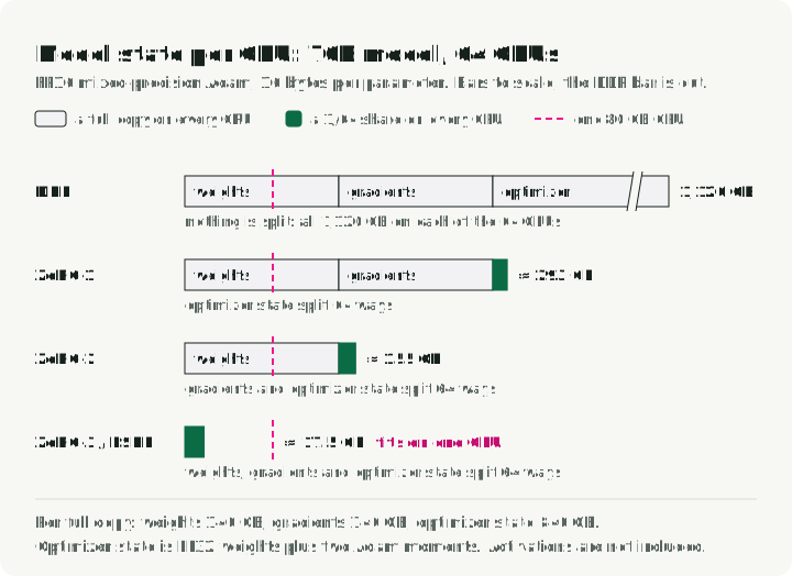
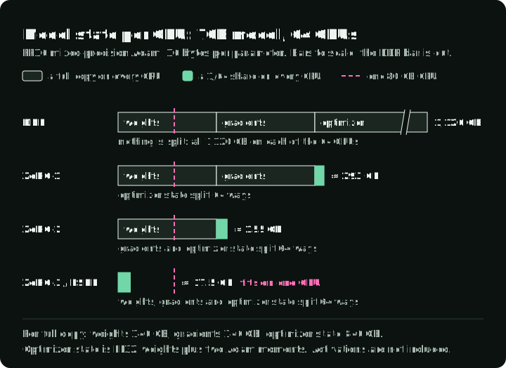
The chart splits each of those four numbers into the part every GPU copies and the part it shares with 63 others, next to the memory of one 80 GB GPU: only full sharding brings model state under it, and the remaining space goes to activations and buffers.
Inference carries no gradients or optimizer state, but it adds the KV cache, which grows with every token the server keeps in memory:
KV bytes per token = 2 × layers × KV heads × head dimension × bytes per valueThe 2 counts keys and values. For Llama 3.1 70B in BF16 (80 layers, 8 KV heads, head dimension 128), that is about 0.33 MB per token, so one sequence of 32,768 tokens holds about 10.7 GB of cache. Multiply by the number of concurrent sequences to size a server. Cache policy, sequence length, concurrency, and quantization change this number.
Memory relief is not a fixed multiplier. The numbers above exclude activations, temporary and communication buffers, and allocator headroom. Real relief depends on sharding degree, what remains replicated, transient unsharded state, activation policy, padding, imbalance, and buffers.
Profile the exact architecture, precision, sequence length, micro-batch, optimizer, checkpointing policy, and runtime. Record peak allocated and reserved memory, tokens per second, time in kernels, and time exposed in collectives. torch.cuda.max_memory_allocated() and torch.cuda.max_memory_reserved() give the two peaks; the PyTorch profiler or Nsight Systems shows kernel time and how much NCCL time is not overlapped with compute.
How ranks communicate
A rank is one training process, usually driving one GPU. Ranks exchange tensors through collectives and point-to-point operations, which the NCCL library implements on NVIDIA GPUs. Five appear in this article; the reduction examples use sums:
- All-reduce: every rank ends with the sum of all ranks’ tensors.
- All-gather: every rank ends with every rank’s shard.
- Reduce-scatter: each rank ends with the sum of one shard.
- All-to-all: each rank sends a different piece to every other rank.
- Point-to-point: one rank sends a tensor to one other rank.
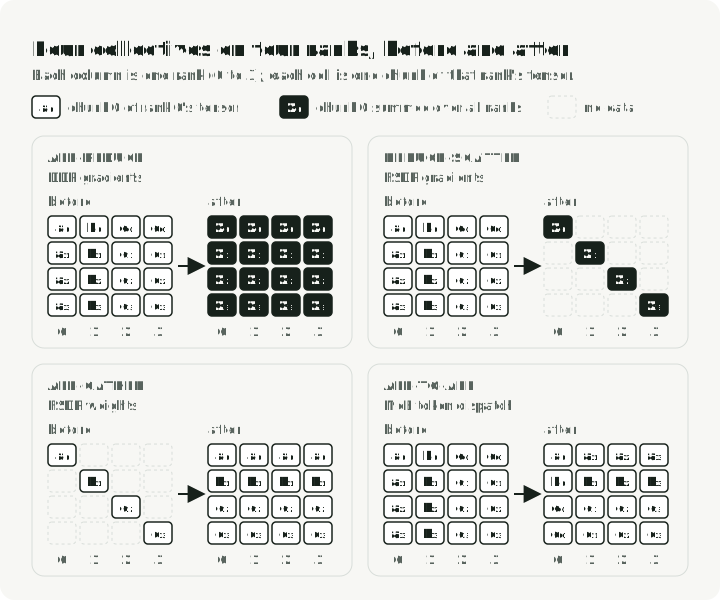
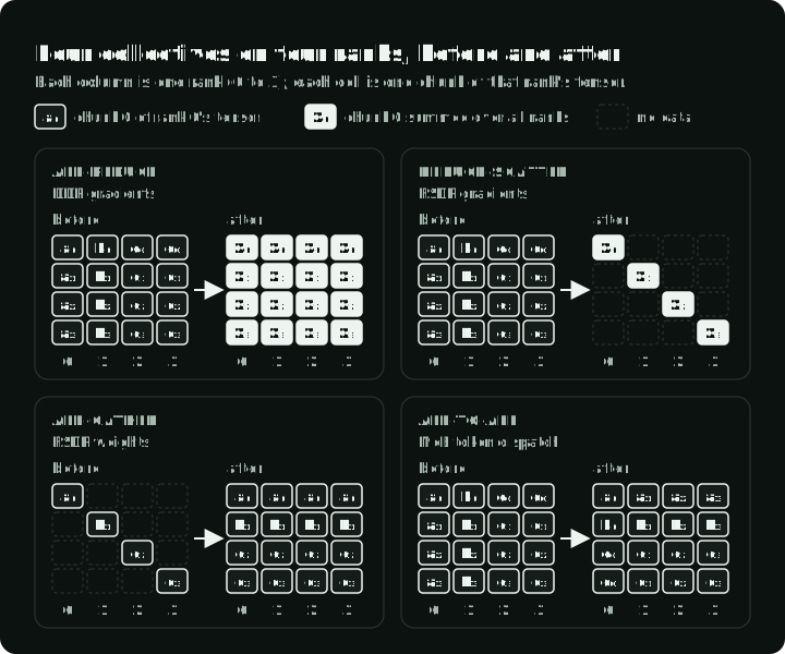
The figure shows four ranks before and after each of the first four operations, one column per rank and one cell per chunk of its tensor. Compare all-reduce with reduce-scatter: both sum across ranks, but reduce-scatter leaves each rank with only its own shard of the sum.
What each strategy splits and communicates
For each strategy, ask which tensor dimension is split, which state is replicated, and which collective enters the critical path.
| Strategy | Splits | Primary relief | Communication introduced |
|---|---|---|---|
| Replicated data parallelism (DDP) | batch | training throughput | gradient all-reduce |
| Fully sharded data parallelism (FSDP) | parameters, gradients, optimizer state across a data-parallel (DP) group | model-state memory | parameter all-gather, gradient reduce-scatter |
| Tensor parallelism (TP) | matrix or attention dimensions inside layers | layer weights and activations | collectives within transformer blocks |
| Pipeline parallelism (PP) | layer groups | model depth and per-stage state | point-to-point activations plus scheduling bubbles |
| Context parallelism (CP) | sequence dimension | long-sequence activation memory | key/value or attention exchange across the sequence group |
| Expert parallelism (EP) | MoE experts and routed tokens | expert capacity per rank | token dispatch and combine, commonly all-to-all |
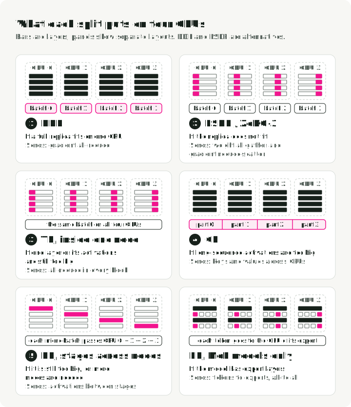
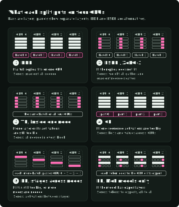
The figure shows six separate layouts on four GPUs. Choose DDP when a full training replica fits with headroom, or FSDP/ZeRO when model state needs sharding. Add other splits only for the constraints they address; the panels do not show those combinations. The sections below explain each split.
Data parallelism (DDP)
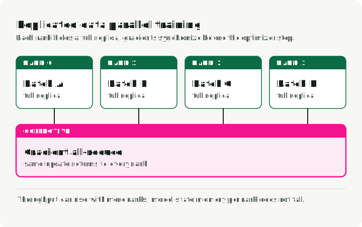
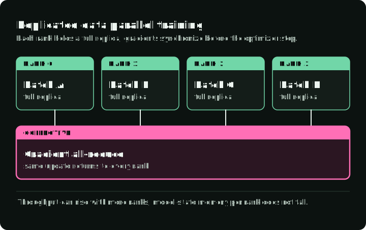
Replicated data parallelism, usually called distributed data parallel, keeps a full training replica on every rank. PyTorch’s DistributedDataParallel documentation describes this replica-and-gradient-synchronization model. Each rank handles a different micro-batch, and gradients are synchronized before the optimizer step.
Use it when the full training state fits with headroom. Each new rank adds its micro-batch to the global batch, so either your training recipe tolerates a larger global batch, or you reduce gradient accumulation to keep it constant. Its main advantages are simple semantics and a mature implementation that overlaps backward computation with bucketed gradient reduction.
Adding ranks can hurt when the local batch becomes too small. It can also hurt when the network cannot hide the all-reduce or input delivery stalls. Larger global batches can give diminishing improvements in time to a target loss while consuming more compute. Compare loss and elapsed time for your training recipe.
The figure shows one training step on one rank. Buckets of gradients are all-reduced while backward runs, and the GPU waits only for the part of the all-reduce the network cannot hide.
In PyTorch you wrap the model in DistributedDataParallel and start one process per GPU with torchrun, which sets RANK, LOCAL_RANK, and WORLD_SIZE for each process. Hugging Face Accelerate launches the same setup from a config file.
Fully sharded data parallelism (FSDP, ZeRO)
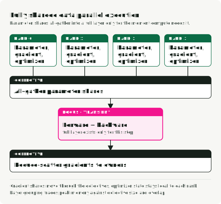
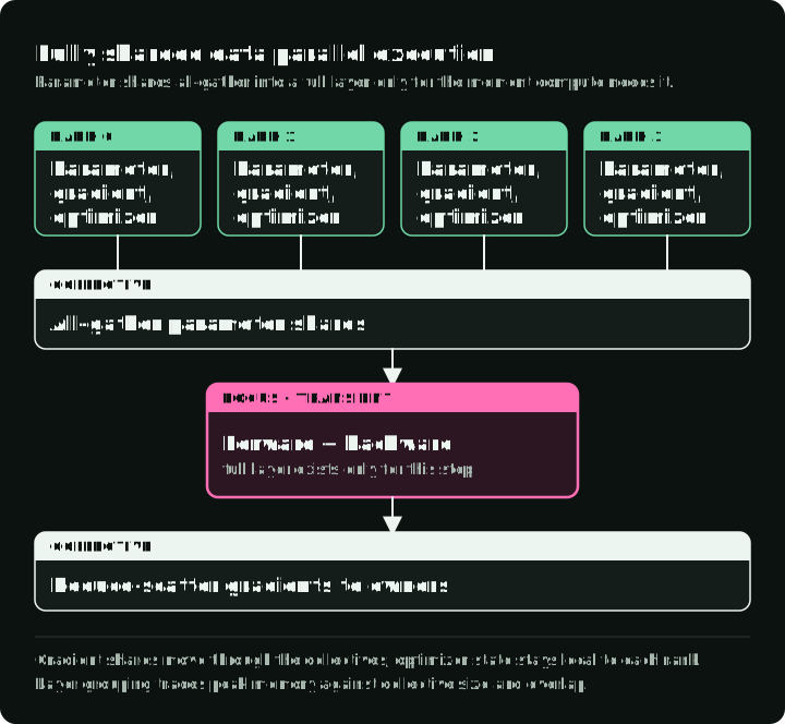
Fully sharded data parallelism stores parameter, gradient, and optimizer shards across a group. The ZeRO paper describes this state-sharding pattern, and PyTorch’s FSDP2 API implements it. A layer’s parameters are all-gathered for computation and can be resharded afterward. Gradients are reduce-scattered back to owners. The figure follows one layer on one of four ranks through a training step: the rank stores a quarter of the weights, gradients, and optimizer state, an all-gather builds the full weights for the forward pass and again for the backward pass, and the reduce-scatter leaves the rank its quarter of the gradients.
The ZeRO paper puts the cost of stage 3 at about 1.5 times the communication volume of DDP: parameters are all-gathered in both the forward and the backward pass, and gradients are reduce-scattered once.
Current PyTorch documentation distinguishes the fully_shard API in fully sharded data parallelism version 2 (FSDP2) from the older FullyShardedDataParallel wrapper. FSDP2 groups communication by the modules to which fully_shard is applied and recommends bottom-up application so layer groups can overlap communication and computation.
The order of calls is the part that is easy to get wrong. This excerpt shards a stack of Transformer layers with FSDP2:
model = nn.Sequential(*layers).cuda()  # e.g. 24 Transformer layers

for layer in model:  # bottom-up: each layer becomes one communication group
    fully_shard(layer)
fully_shard(model)  # then shard the remaining root parameters

# Build the optimizer after sharding, so it holds the sharded parameters (DTensors).
optimizer = torch.optim.AdamW(model.parameters(), lr=1e-4)
Launch one process per GPU with torchrun --nproc_per_node=8 train.py. Peak memory per rank falls as the shard group grows, because each rank keeps a smaller share of the FP32 weights, gradients, and Adam state. Activations do not shrink, because each rank still processes its own batch. The FSDP2 tutorial has a complete script with mixed precision and checkpointing. FSDP2 also has a reshard_after_forward=False option that keeps parameters gathered between the forward and backward pass. It behaves like ZeRO-2: fewer all-gathers, more memory.
Sharding is attractive when model state is the largest part of memory and layer compute can hide enough collective traffic. It may be a poor trade for small models, slow links, tiny layers, or a shard group that spans nodes over a slow network. DeepSpeed ZeRO implements the same stages with explicit stage selection and optional offload of state to CPU or NVMe memory.
Tensor parallelism
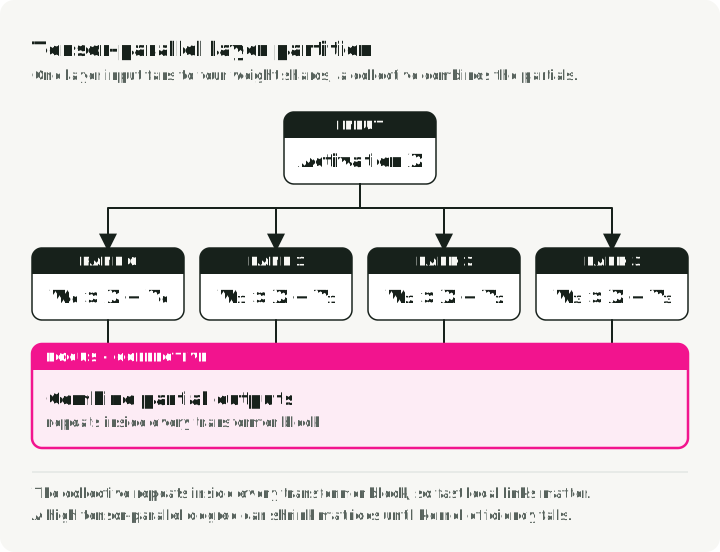
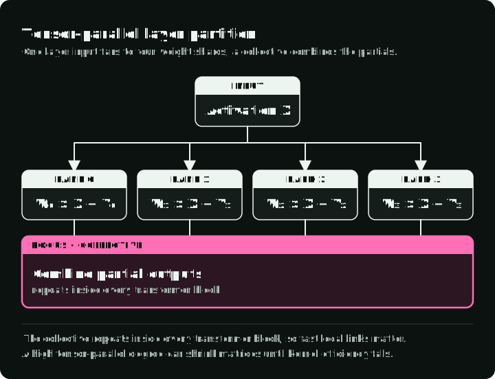
Tensor parallelism partitions linear algebra inside a layer. Examples include column-parallel and row-parallel projections. NVIDIA’s parallelism guide documents this layer-level split. Partial results require collectives within transformer blocks, so latency and bandwidth matter repeatedly throughout the forward and backward passes.
The figure shows the split the Megatron-LM paper uses for a Transformer MLP on two ranks. The first weight matrix is split by columns, so each rank applies GeLU to its own slice with no communication. The second matrix is split by rows, so each rank produces a partial sum of the output, and one all-reduce adds them. That is one all-reduce per MLP in the forward pass instead of one per matrix multiplication.
Use it when a layer or its activations do not fit, or when the matmuls are large enough for partitioned kernels to outperform one rank. Map the tensor-parallel group to the fastest communication domain available, then measure. A high tensor-parallel degree can shrink each local matrix until kernel efficiency falls while collective overhead grows.
Megatron-style sequence parallelism splits the activations of the LayerNorm and dropout regions along the sequence, which plain TP would otherwise keep in full on every rank in the TP group. It works inside the TP group; context parallelism splits the whole sequence, including attention, across a separate group.
Megatron Core implements TP and sequence parallelism for training. vLLM, SGLang, and TensorRT-LLM use TP to shard a model for serving.
Pipeline parallelism
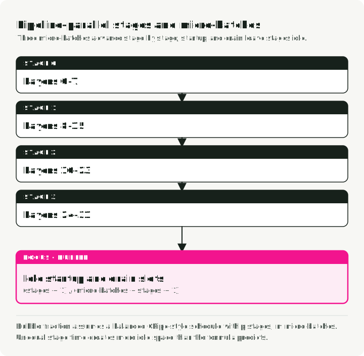
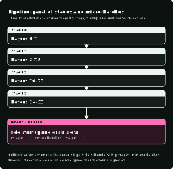
Pipeline parallelism places different layer groups on different stages and sends activations between them. Micro-batches keep stages working concurrently.
It relieves per-stage model state and can reduce the volume of communication crossing a slower boundary compared with per-layer tensor collectives. Its costs are bubbles, activation transfers, stage imbalance, more complex scheduling, and harder recovery and checkpointing.
The figure shows the forward pass of four stages and four micro-batches over seven time steps, and below it the idle share for more micro-batches. Each empty slot is a stage with no work: the last stages wait at the start, and the first stages wait at the end. For a simple balanced GPipe-style schedule with p stages and m micro-batches, the idealized forward bubble fraction is approximately:
(p - 1) / (m + p - 1)With 4 stages, 4 micro-batches leave 3/7, about 43%, of the forward schedule idle. 16 micro-batches leave 3/19, about 16%, and 32 leave 3/35, about 9%. More micro-batches per global batch shrink the bubble, but each one is smaller, so kernels run less efficiently; measure both.
Real schedules may use one-forward/one-backward, interleaving, or zero-bubble variants, and unequal layer cost can dominate the formula. Choose stage boundaries from measured time and memory, not equal layer counts.
DeepSpeed, Megatron Core, and Nanotron implement pipeline schedules.
Context parallelism
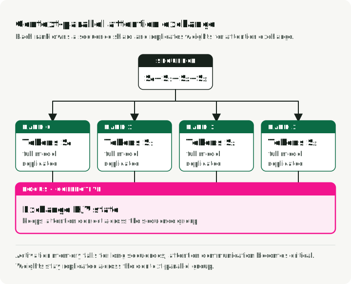
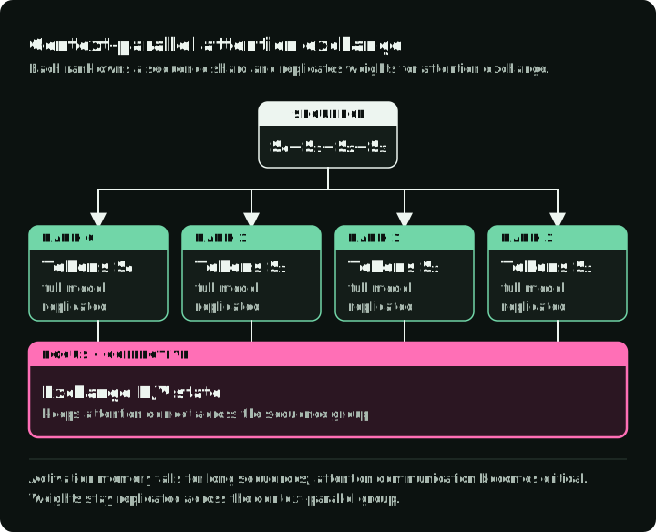
Context parallelism distributes the sequence dimension. NVIDIA’s context parallelism documentation describes the sequence split and the key/value exchange needed for attention. Each rank owns a sequence shard, while attention exchanges the information needed to preserve full-context semantics. Implementations may use point-to-point rings, all-gather, all-to-all, or hierarchical combinations.
It reduces activation memory for long-context training but replicates weights across the context group and introduces attention communication. Benefit depends on attention type, causal masking, sequence length, recomputation, and how context groups compose with tensor and data parallel groups.
Do not select it from a universal 8K, 32K, or 100K threshold. Consider it when activations still exceed memory at your target sequence length after activation checkpointing and tensor plus sequence parallelism, and the weights already fit.
Megatron Core implements CP for training. Picotron has a small implementation of data, tensor, pipeline, and context parallelism for learning how they fit together.
Expert parallelism for MoE models
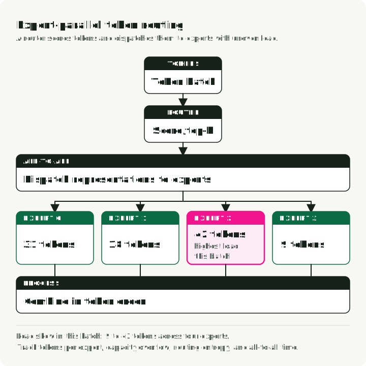
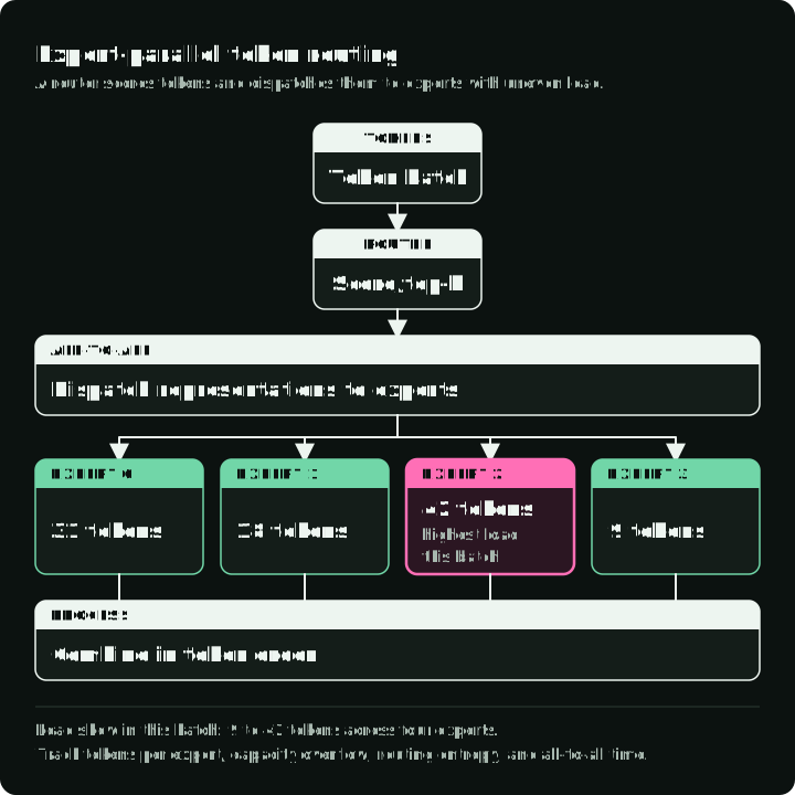
Expert parallelism distributes experts in mixture-of-experts layers. Mixtral 8x7B, for example, stores about 46.7B parameters but uses about 12.9B per token. NVIDIA’s parallelism guide documents this expert placement and its combination with other parallel dimensions. The router sends token representations to selected experts and combines their results. Only selected experts compute for each token, but total expert weights still require storage and serving placement.
Expert parallelism is not an optimization switch for a dense model. It is part of an MoE architecture. Its concerns include load balance, capacity limits, token all-to-all, dropped tokens, padding, auxiliary losses, and failure skew. Megatron’s MoE settings distinguish dropping assignments above an expert’s capacity from padding unused slots below it. Dropless routing processes variable token counts. Track tokens per expert, routing entropy, capacity overflow, communication time, and quality by route.
Megatron Core and Nanotron implement EP for training.
Compose a layout from the topology
Large dense-model training systems with no expert-parallel group commonly use a product of data-parallel (DP), tensor-parallel (TP), pipeline-parallel (PP), and context-parallel (CP) group sizes:
world size = DP × TP × PP × CPWhen expert parallelism (EP) is an independent group, NVIDIA’s parallelism guide calculates the total as:
total GPUs = TP × PP × CP × EP × DPCheck which group orders and sizes your framework supports before choosing degrees.
Build the layout in this order:
- Draw communication domains: GPU-to-GPU links, switches, non-uniform memory access (NUMA) boundaries, node fabric, oversubscription, and storage path. On most GPU servers the fastest domain is NVLink between the GPUs of one node; nodes connect over a slower network such as InfiniBand.
- Place frequent latency-sensitive collectives, commonly TP, in the fastest suitable domain. This usually means keeping each TP group inside one node.
- Choose FSDP or replicated DP groups from remaining capacity and bandwidth.
- Add PP when depth placement or cross-domain traffic benefits, balancing measured stage time and memory.
- Add CP only for the sequence constraint, and EP only for the model’s expert topology.
- Confirm divisibility of heads, hidden dimensions, layers, experts, batch, and sequence for the candidate mesh.
- Benchmark several valid meshes. Topology-aware heuristics choose candidates, not winners.
An example candidate for a dense 70B model with 32K context on 64 nodes of 8 GPUs: TP=8 inside each node over NVLink, PP=4 across nodes, CP=4 for the long sequence, and DP=4 for the rest; 8 × 4 × 4 × 4 = 512 GPUs. Benchmark it against TP=8, PP=8, CP=2, DP=4 before choosing.
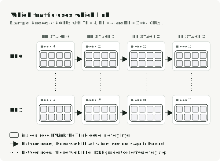
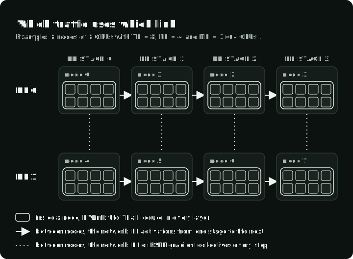
The figure shows where each group’s traffic goes in that kind of layout: the TP all-reduce stays on NVLink inside a node, while FSDP or DP gradient collectives and PP activations cross the network between nodes.
Starting candidates by cluster size, to benchmark rather than adopt:
- One node, 2–8 GPUs. DDP when a full training replica fits with headroom; FSDP2 or DeepSpeed ZeRO-2/3 when model state needs sharding. Launch with
torchrunor Accelerate. Add TP=2 only if one layer or its activations still do not fit. On PCIe-connected GPUs without NVLink, keep TP at 1 or 2, because every layer’s all-reduce crosses PCIe. - 2–16 nodes. TP inside each node (4 or 8 with NVLink), FSDP or DP across nodes, and PP across nodes only if the model still does not fit.
- Hundreds of GPUs or more. TP × PP × CP × DP, as in the example above, with a framework that implements all four, such as Megatron Core.
Two clusters with the same GPU count can prefer different layouts because link bandwidth, switch hierarchy, CPU attachment, and network contention differ.
Which framework implements which split
The splits above are implemented by a small set of libraries. Pick by the splits you need and how much of the training loop you want to own.
| Tool | Splits it supports | Use it when |
|---|---|---|
| Hugging Face Accelerate | launches DDP, FSDP, or DeepSpeed from a config file | you want an existing PyTorch or Transformers script on several GPUs with few code changes |
| PyTorch DDP and FSDP2 | DDP, FSDP (fully_shard), with torchrun | you train a dense model on one node or a few nodes and want plain PyTorch |
| DeepSpeed ZeRO | ZeRO stages 1, 2, 3, CPU and NVMe offload, PP | you want to choose the sharding stage, or offload state to CPU or NVMe memory |
| Megatron Core | TP, PP, CP, EP, DP, and sequence parallelism | you need TP, PP, and CP (and EP) together for large pretraining runs |
| Nanotron | DP, TP, PP, EP, ZeRO-1 | you want a smaller codebase than Megatron for 3D parallelism and MoE |
| vLLM, SGLang, TensorRT-LLM | TP and PP for inference | you serve the model; see the serving section below |
To run an existing script with FSDP2 through Accelerate, run accelerate config once; it writes the config file interactively. These settings select FSDP2, decoder-layer grouping, and resharding:
fsdp_config:
    fsdp_version: 2
    fsdp_auto_wrap_policy: TRANSFORMER_BASED_WRAP
    fsdp_transformer_layer_cls_to_wrap: LlamaDecoderLayer
    fsdp_reshard_after_forward: true
With fsdp_auto_wrap_policy: TRANSFORMER_BASED_WRAP, fsdp_transformer_layer_cls_to_wrap names the block class that becomes one FSDP unit, the same bottom-up grouping as the fully_shard loop above. fsdp_reshard_after_forward: true is full sharding; false is the ZeRO-2-like mode. Start the job with accelerate launch --config_file fsdp2.yaml train.py. The FSDP1/FSDP2 guide explains these version-specific settings and the accelerate to-fsdp2 command that converts an older FSDP1 config.
Training and serving need separate decisions
Inference usually does not carry gradients or optimizer state, so FSDP-style training layouts do not transfer automatically.
Prefill processes the prompt and stores its tokens’ keys and values in the KV cache. Decode generates subsequent tokens while reusing and extending that cache.
For serving, ask:
- Does one replica fit weights, KV cache, workspace, and target concurrency?
- Is throughput better served by more independent replicas or by sharding one replica?
- Does TP reduce per-rank weight and cache pressure enough to repay per-layer communication?
- Is PP supported efficiently for the model and request scheduler?
- How do prefill and decode stress compute, memory bandwidth, and interconnect differently?
- What happens to tail latency when requests have different prompt and output lengths?
Use the KV-cache formula from the memory section for the first question. If one replica fits with room for the KV cache at your target concurrency, run more replicas; they need no communication between GPUs. If it does not fit, shard it with TP inside one node first, and add PP across nodes only when one node is not enough. In vLLM these are --tensor-parallel-size and --pipeline-parallel-size; SGLang and TensorRT-LLM have the same two settings.
Benchmark the complete server with the scheduler, quantization, context distribution, batching policy, and traffic shape. Training tokens per second cannot predict serving time to first token or inter-token latency.
What to record for each candidate layout
For each candidate, record:
- model, code, runtime, kernels, and topology identity
- global and local batch, sequence distribution, and token count
- peak memory by category where available
- useful tokens per second and model floating-point operation (FLOP) utilization when calculated consistently
- exposed time in all-reduce, all-gather, reduce-scatter, all-to-all, and point-to-point operations
- input stalls, checkpoint time, restart behavior, and straggler distribution
- training loss or serving-output parity against the baseline
Compare weak and strong scaling deliberately. Strong scaling holds total work constant as rank count increases. Weak scaling holds work per rank constant, so total work grows with rank count. A percentage labeled “scaling efficiency” is meaningless without that denominator and baseline.
Conclusion
Parallelism is a mapping from a measured bottleneck to a tensor dimension and a communication pattern. Replication, sharding, layer partitioning, staging, sequence partitioning, and expert routing each relieve a different constraint and create a different failure mode.
Inventory the workload, draw the topology, generate valid meshes, and profile them. The winning layout is the one that fits with headroom and minimizes exposed communication for the job you run.
References
- PyTorch FSDP2
fully_sharddocumentation - Module-level parameter sharding, all-gathers, reduce-scatters, and DTensor behavior. - PyTorch DistributedDataParallel documentation - Replicated model training with synchronized gradients.
- PyTorch
torchrundocumentation - Launching one process per GPU with rank environment variables. - NVIDIA Megatron Core parallelism strategies - Data, tensor, pipeline, context, expert, and fully sharded strategy dimensions.
- Hugging Face Ultra-Scale Playbook - Interactive overview of large-scale model parallelism.
- Ultra-Scale Playbook cheat sheet - One-page summary of the playbook.
- Hugging Face Accelerate FSDP guide - Config keys and launch commands for FSDP.
- DeepSpeed ZeRO tutorial - ZeRO stages and offload configuration.
- DeepSpeed ZeRO paper - Sharding optimizer states, gradients, and parameters to reduce memory use.
- Megatron-LM paper - Column- and row-parallel Transformer layers.
- Reducing Activation Recomputation in Large Transformer Models - Megatron sequence parallelism.
- GPipe paper - Pipeline training with micro-batches and staged execution.
- vLLM parallelism and scaling - Tensor and pipeline parallel serving settings.
- Mixtral of experts - Total and active parameter counts for Mixtral 8x7B.
- NERSC parallelism documentation - Strong and weak scaling definitions based on fixed total or per-rank work.
