Search Ranking Stack: BM25, Embeddings, and Reranking

This guide is for Python engineers building or improving a search ranking pipeline. It explains how BM25, dense embeddings, rank fusion, and rerankers work together, and how to measure whether search needs better candidates or a better order.
A search for “cheap laptop” can miss a product described as a “budget notebook computer.” A different failure puts a headphone carrying case above the headphones themselves. The first problem needs better candidates; the second needs a better order.
The companion demo repository illustrates retrieval and reranking on a sampled slice of Amazon ESCI product-search data.
For a compact stage-selection guide, see BM25 vs Embeddings vs Rerankers. The experiment sequence later in this article connects each stage to a measurement.
Lexical, dense, and cross-encoder models
The stack is easier to understand as three layers. Lexical retrieval finds exact terms, dense retrieval closes vocabulary gaps, and rerankers compare the strongest candidates in detail.
BM25 and lexical retrieval
For decades, BM25 was the default. It’s a probabilistic model that scores documents by the frequency of query terms in the document, normalized by document length and inverse document frequency (IDF).
BM25 is strong when literal terms carry the intent: error codes, product SKUs, names, and API identifiers. Its main limitation is vocabulary mismatch. A query for “cheap laptop” may miss a document about a “budget notebook computer” when the indexed text provides no bridge between the expressions.
That said, the BEIR study found BM25 a strong zero-shot baseline across its heterogeneous retrieval tasks. BEIR’s BM25 numbers come from Lucene through Pyserini, not from the whitespace-tokenized rank_bm25 used in this demo. BM25 also beats some neural models on argumentative retrieval tasks like Touche-2020.
Dense retrieval and embeddings
BERT-style encoders made dense retrieval practical. They map queries and documents into a shared vector space, then rank candidates with a similarity function such as cosine similarity or dot product.
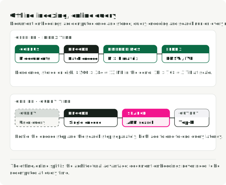
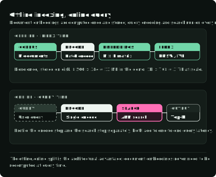
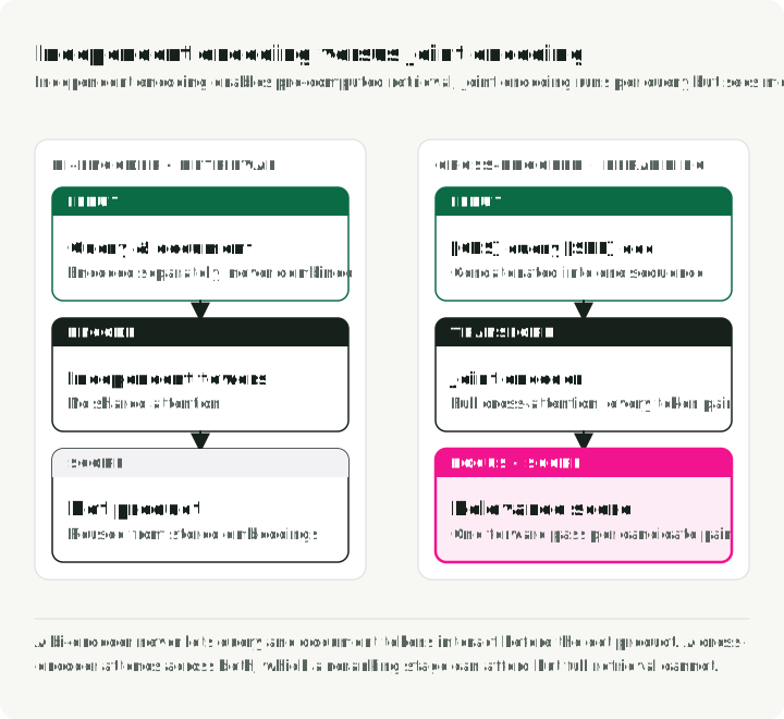
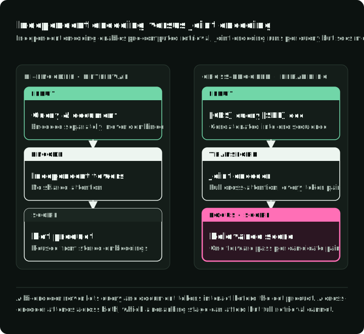
The bi-encoder (or “two-tower”) architecture encodes the query and the document separately, producing fixed-length embeddings. Document vectors can be pre-computed and indexed offline, then retrieved fast via Approximate Nearest Neighbor (ANN) algorithms. Now “cheap laptop” and “budget notebook” land close together in vector space.
Some bi-encoders use a Siamese architecture, as in Sentence-BERT, where both sides share weights. Others use separate query and document towers. Pooling, vector size, similarity function, and training objective are model choices rather than properties of every dense retriever.
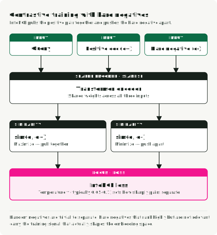
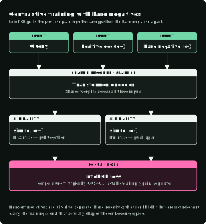
These models are trained with contrastive learning, usually with the InfoNCE loss. Given a batch of (query, positive_document) pairs, the objective maximizes sim(query, positive_doc) while minimizing sim(query, negative_docs). Negatives come from other queries’ positives in the same batch (in-batch negatives). A temperature parameter controls how sharply the model has to separate the two.
Training data often matters more than the embedding dimension. Retrieval models learn from query-positive pairs and carefully selected hard negatives: plausible but non-relevant documents. The later training section shows how SimANS avoids both trivial negatives and likely false negatives.
The cost is the representation bottleneck. Bi-encoders compress all semantic nuance into a single fixed-size vector, so they often miss fine-grained interactions between specific query terms and specific document content.
Cross-encoders and LLMs
Cross-encoders (Nogueira & Cho, 2019) feed the query and document into a Transformer together as a concatenated sequence ([CLS] Query [SEP] Document), so every query token can attend to every document token through full self-attention. That deep interaction picks up nuance that independent encoding misses.
LLM reranking uses a prompted model to compare several candidates at once. RankGPT showed strong zero-shot listwise results with GPT-4 on its evaluated benchmarks, but output stability, cost, and domain fit still need separate testing.
These scores cannot be pre-computed for arbitrary queries, so reranking is placed after retrieval. That cost asymmetry motivates the multi-stage funnel.
The multi-stage funnel
Running an expensive cross-encoder or LLM across millions of documents isn’t viable, so modern search stacks use a funnel. Retrieval and pre-ranking reduce the candidate pool so full ranking can use more expensive models on a shortlist. Blending then applies rules or a ranking policy; its cost depends on that policy.
A cheap retriever also lacks final precision, so the funnel uses each model only where its cost is reasonable. The figure shows each stage’s input volume and schematic model cost, and marks that later stages cannot recover omitted documents:
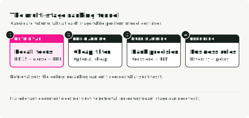
| Stage | Input scale | Primary objective | Typical methods | Exit measurement |
|---|---|---|---|---|
| Retrieval | Corpus or index | Candidate recall | BM25, bi-encoders | Recall at candidate cutoff |
| Pre-ranking | Large candidate set | Cheap filtering | Lightweight models, rules | Recall retained per millisecond |
| Full ranking | Shortlist | Top-rank quality | Cross-encoders, LLMs | NDCG/MRR, latency, cost |
| Blending | Final ranked lists or slots | Constraints and mix | Rules, multi-objective rank | Policy, diversity, business guardrails |
A reranker reorders the candidates retrieval returns; it cannot add one. Retrieved candidate coverage therefore limits what later stages can recover. With more than 100 candidates, reranking can move a relevant document into the top 100 and improve Recall@100. In this demo, all 100 candidates remain, so reranking cannot change Recall@100.
Tools for each stage
The demo uses small in-memory libraries. Outside a laptop, each stage has a few common implementations:
| Stage | Tool | Use when |
|---|---|---|
| BM25 | rank_bm25 | The corpus fits in memory and you want a quick baseline |
| Elasticsearch, OpenSearch, or Lucene through Pyserini | The corpus needs an inverted index, analyzers, and filters | |
| Dense retrieval | FAISS | You want an ANN library inside your own service |
| pgvector | The data already lives in Postgres | |
| Qdrant, Weaviate, Vespa, or Elasticsearch kNN | You need metadata filters, frequent updates, and a managed index | |
| Fusion | Elasticsearch RRF retriever, Qdrant Query API with rrf | You want rank fusion inside the search engine |
| Weaviate hybrid search | You use Weaviate; it offers ranked fusion and relative-score fusion | |
| Embedding models | The MTEB retrieval tab, then your own judged queries | You are choosing a model; the leaderboard narrows the list, your queries decide |
| Reranker | ms-marco-MiniLM-L12-v2 | English text, CPU budget |
bge-reranker-v2-m3 | Multilingual text | |
| Elastic Rerank | English text already in Elasticsearch; it needs an eligible subscription or a trial |
The demo: a five-stage pipeline
To make this concrete, I built a search-ranking-stack demo that runs a five-stage pipeline on the Amazon ESCI product search benchmark. Each stage writes metrics.
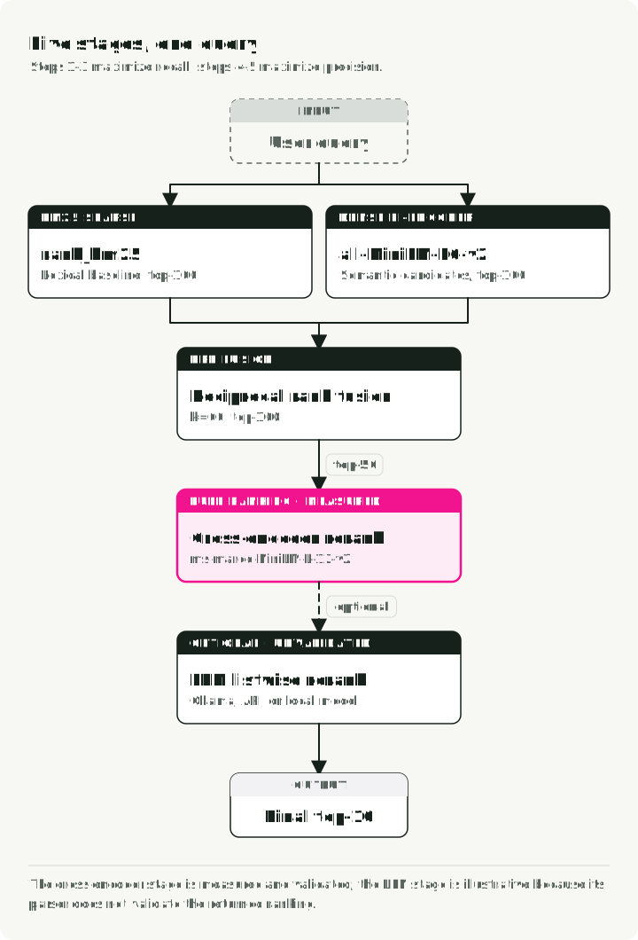
The pipeline:
- BM25 sparse retrieval — lexical baseline (
rank_bm25) - Dense bi-encoder retrieval — semantic candidate generation (
all-MiniLM-L6-v2) - Hybrid RRF fusion — rank-based fusion of sparse and dense results
- Cross-encoder reranking — pairwise relevance scores (
ms-marco-MiniLM-L12-v2) - LLM listwise reranking — prompted comparison of the final shortlist (Ollama, API, or local model)
Steps 1—3 are the retrieval stage of the funnel (maximize recall); steps 4—5 are the full ranking stage (maximize precision). The demo skips pre-ranking and blending. The diagram shows the candidate count at each step: the cross-encoder scores the first 50 of 100 hybrid candidates and keeps the rest in hybrid order, and the LLM sees the first 10.
Quick start
The download step fetches the dataset once and writes a small sample. run-all then runs every stage, prints one metrics row per stage, and writes the rows to results/metrics.json and a chart to results/metrics_comparison.png. Add --llm-mode to include the LLM stage.
git clone https://github.com/slavadubrov/search-ranking-stack.git
cd search-ranking-stack
uv sync

# Download and sample ESCI dataset (~2.5GB download, ~5MB sample)
uv run download-data

# Run BM25, dense, hybrid RRF, and the cross-encoder
uv run run-all

# Add LLM reranking with a local Ollama model (ollama pull llama3.2:3b first)
uv run run-all --llm-mode ollama
Dataset and sampling: Amazon ESCI
The demo uses the Amazon Shopping Queries Dataset (ESCI) from KDD Cup 2022 — a real product search benchmark with four-level graded relevance labels:
| Label | Gain | Meaning | Example (Query: “wireless headphones”) |
|---|---|---|---|
| Exact (E) | 3 | Satisfies all query requirements | Sony WH-1000XM5 Wireless Headphones |
| Substitute (S) | 2 | Functional alternative | Wired headphones with Bluetooth adapter |
| Complement (C) | 1 | Related useful item | Headphone carrying case |
| Irrelevant (I) | 0 | No meaningful relationship | USB charging cable |
Graded relevance matters because it lets you use NDCG (Normalized Discounted Cumulative Gain), which separates a “perfect” ranking from a “merely adequate” one. Binary metrics score both the same.
I used the demo’s small_version sample: 500 queries, 9,870 products, and 9,984 judgments. Its downloader reads tasksource/esci’s single train split, filters the English us locale and small_version == 1, then uses seed 42 to sample up to 500 unique query IDs without replacement. The corpus contains the unique products from those selected judgment rows. This is not a held-out split or an independent corpus. The sample is small enough to run on a laptop, but too small and domain-specific to establish a production ranking. Use it to reproduce the stages and inspect failure modes; use held-out, representative queries to make deployment decisions.
Evaluation: measuring what matters
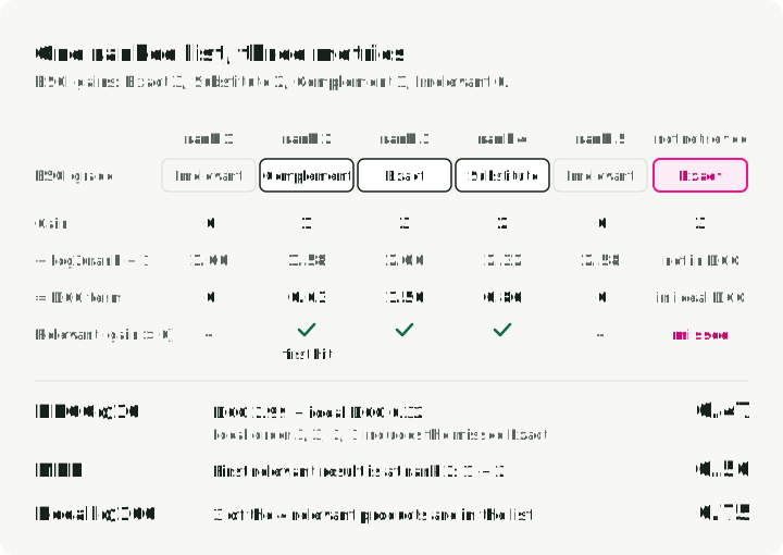
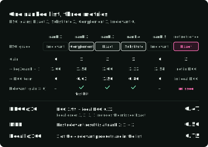
The demo uses three metrics, each looking at the ranking from a different angle. The figure applies all three to one query’s results, using the ESCI gains above:
NDCG@10 (primary metric)
Normalized Discounted Cumulative Gain measures the quality of the top-10 ranking using graded relevance. It rewards placing highly relevant documents near the top with a logarithmic discount:
This matches the linear gains used by trec_eval’s ndcg_cut, selected through pytrec_eval as ndcg_cut_10. IDCG is the DCG of the ideal ordering of the judged grades; a query with no positive gain receives zero. Exponential gains such as define a different convention and would change these numbers.
Of the three, NDCG is the only metric that fully uses ESCI’s four-level graded relevance. A system that places an Exact match at position 1 scores higher than one that places a Substitute there. That’s why it’s the primary metric here.
MRR (first Complement-or-higher result)
Mean Reciprocal Rank uses the position of the first result counted as relevant. In this demo, the evaluator passes ESCI’s relevance judgments to pytrec_eval and uses recip_rank over each returned list of up to 100 candidates. Its binary threshold is relevance > 0: Complement (1), Substitute (2), and Exact (3) count as relevant. Irrelevant (0) does not. A relevant result at position 1 gives reciprocal rank 1.0; at position 3, it is 0.333. This is MRR over the returned candidate lists, not MRR@10.
Recall@100 (retrieval coverage)
Recall@100 measures what fraction of judged relevant documents appear in the top 100. It stays fixed when reranking the same 100 candidates, as in this demo. With a larger candidate pool, reranking can move a relevant document into the top 100 and raise the metric, but it cannot recover a document retrieval omitted.
The denominator includes only judged relevant documents, as in trec_eval’s recall implementation. An unjudged product contributes no positive relevance and is absent from that denominator. Incomplete judgments can therefore make measured recall differ from coverage of all truly relevant products.
Retrieval: hybrid search
The retrieval layer’s job is to maximize recall: get as many relevant documents as possible into the candidate set.
BM25: the lexical baseline
BM25 scores documents by term overlap with the query, with term frequency saturation and document length normalization:
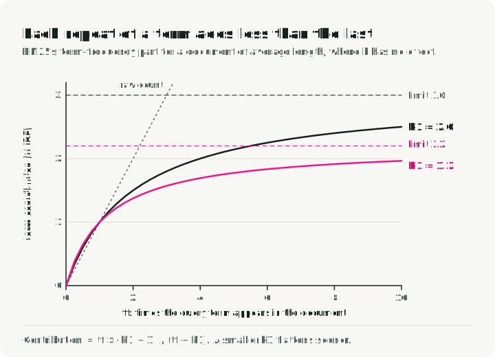
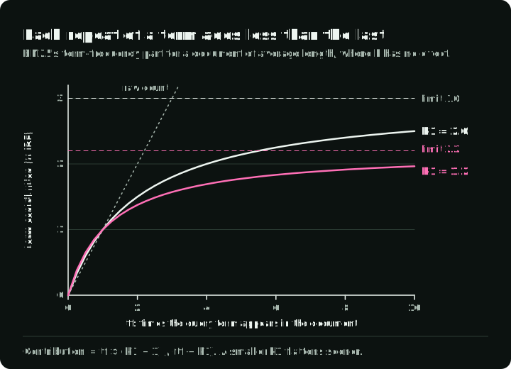
Where is the inverse document frequency of term , is the term frequency in document , is document length, and is the average document length across the corpus. Two parameters matter: (typically 1.2—2.0) controls TF saturation — how quickly repeated terms stop adding value — and (typically 0.75) controls document length normalization.
The chart plots the term-frequency part of the formula for both ends of the usual range:
The implementation is short. Plain whitespace tokenization with rank_bm25:
# src/search_ranking_stack/stages/s01_bm25.py

from rank_bm25 import BM25Okapi

def run_bm25(data: ESCIData, top_k: int = 100):
    doc_ids = list(data.corpus.keys())
    tokenized_corpus = [text.lower().split() for text in data.corpus.values()]

    bm25 = BM25Okapi(tokenized_corpus)

    results = {}
    for query_id, query_text in data.queries.items():
        scores = bm25.get_scores(query_text.lower().split())
        top_indices = np.argsort(scores)[::-1][:top_k]
        results[query_id] = {doc_ids[idx]: float(scores[idx]) for idx in top_indices}

    return results
BM25 lands at Recall@100 of 0.741 — 74% of judged relevant products show up somewhere in the top 100. A reranker given only that BM25 list cannot recover the missing 26% of judged relevant items.
Dense bi-encoder retrieval
The bi-encoder maps queries and documents independently into a shared embedding space:
# Simplified from src/search_ranking_stack/stages/s02_dense.py

import numpy as np
from sentence_transformers import SentenceTransformer

model = SentenceTransformer("sentence-transformers/all-MiniLM-L6-v2")
doc_texts = ["Sony WH-1000XM5 Wireless Headphones", "Headphone carrying case"]
query_texts = ["wireless headphones"]

# Encode corpus once, cache to disk
corpus_embeddings = model.encode(
    doc_texts,
    batch_size=128,
    normalize_embeddings=True,  # Cosine sim = dot product
    convert_to_numpy=True,
)

# At query time: encode query, compute dot product
query_embeddings = model.encode(query_texts, normalize_embeddings=True)
similarity_matrix = np.dot(query_embeddings, corpus_embeddings.T)
With normalized embeddings, cosine similarity reduces to a dot product. The demo computes the full query-by-corpus matrix because 9,870 documents fit comfortably in memory; a production corpus would normally use an approximate-nearest-neighbor index. In this sample, all-MiniLM-L6-v2 raises Recall@100 from 0.741 to 0.825.
How bi-encoders learn good representations
Encoder pretraining and embedding fine-tuning solve different problems. A pretrained Transformer supplies token representations; contrastive fine-tuning teaches a pooled vector which texts should be close. NLI, sentence similarity, and query-passage data are possible ingredients, not a universal sequence. The demo’s all-MiniLM-L6-v2 model card describes a pretrained MiniLM encoder fine-tuned on more than one billion heterogeneous sentence pairs.
Retrieval fine-tuning can use hard negative mining. Random negatives, such as a cooking document paired with a headphones query, may be too easy to teach much. A retriever can instead supply plausible candidates that the judgments identify as non-relevant. Unjudged high-scoring documents need care: some may be missing positives.
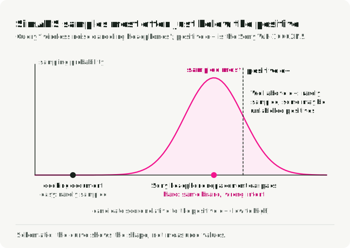
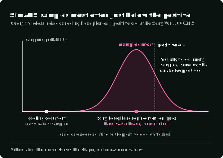
SimANS samples negatives with a probability distribution concentrated near the positive document’s relevance score. It reduces the emphasis on both easy negatives and the highest-scoring candidates that may be false negatives. This is biased sampling from retrieved candidates, not a hard rule that excludes every document above or below a rank boundary. The curve shows how often a retrieved candidate is sampled, by its score relative to the positive:
# What a training triplet looks like after hard negative mining
training_triplet = {
    "query": "wireless noise canceling headphones",
    "positive": "Sony WH-1000XM5 Wireless Noise Cancelling Headphones",
    "negative": "Sony headphone replacement ear pads",  # Hard negative: same brand, related product, but wrong intent
}
# The bi-encoder must learn that "ear pads" is NOT what the user wants,
# even though it shares many tokens with the positive document.
The contrastive loss function (InfoNCE) ties this together. For each query with positive document and a set of negative documents :
Where is cosine similarity between query and document embeddings, and is the temperature parameter (typically 0.05—0.1). Lower values make the loss more sensitive to hard negatives. It is a softmax cross-entropy: push the positive pair’s similarity up relative to all negatives. When is small, even slight differences in similarity produce large gradients, which forces the model into finer-grained distinctions.
Serving bi-encoder embeddings at scale
The architectural advantage of a bi-encoder is the offline/online split. Document embeddings are computed at index time and stored in a vector index. At query time, the system encodes the query and searches those stored vectors. Latency depends on the encoder, hardware, index, filters, and recall target, so profile the two steps separately.
In the demo, the math is modest: 9,870 documents 384 dimensions 4 bytes per float = ~15 MB of embeddings. At production scale the numbers stop being modest: 1 billion documents with 768-dimensional embeddings need ~3 TiB of storage. That’s where quantization (compressing 32-bit floats to 8-bit integers), product quantization (decomposing vectors into subspaces), and SSD-backed indexes like DiskANN come in. The dense-vector indexing section covers the index algorithms.
Why test hybrid retrieval
The two methods often fail differently. BM25 is well suited to proper nouns, product SKUs, and error codes. Dense retrieval can recover vocabulary mismatch such as “cheap laptop” versus “budget notebook computer.” Whether fusion helps depends on how often those complementary cases occur in the target query set.
A common next experiment is hybrid search: run both retrieval methods, then fuse their ranked lists.
Reciprocal rank fusion (RRF)
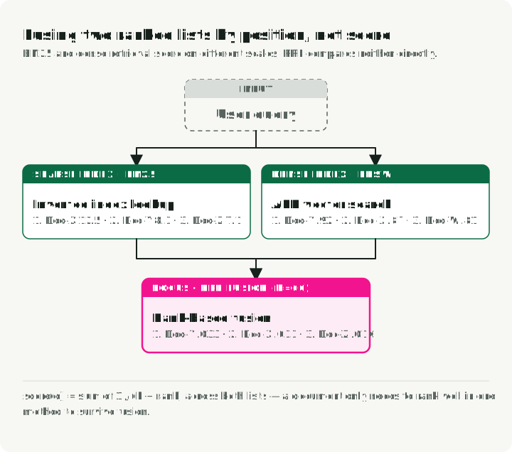
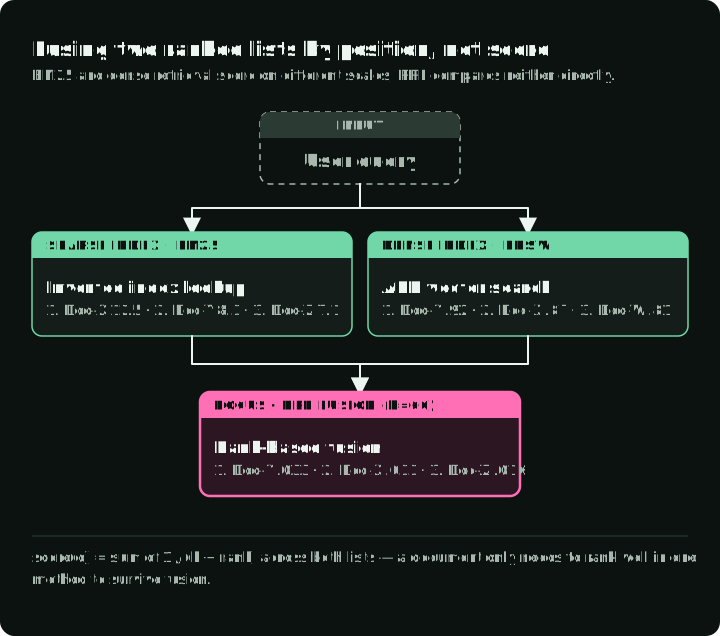
BM25 and dense retrieval produce scores with different meanings and scales. A linear combination therefore needs calibration and validation whenever the retrievers or corpus change.
Reciprocal Rank Fusion (Cormack et al., 2009) drops raw scores entirely and uses only the rank position:
Here, is a smoothing constant; 60 is a common starting value. RRF rewards items that rank near the top across input lists without comparing their raw scores. It avoids score-scale calibration, but the retrieval cutoffs, weights, and still require evaluation.
The implementation:
# src/search_ranking_stack/stages/s03_hybrid_rrf.py

from collections import defaultdict

def reciprocal_rank_fusion(ranked_lists, k=60, top_k=100):
    all_query_ids = set().union(*(results.keys() for results in ranked_lists))
    fused_results = {}

    for query_id in all_query_ids:
        rrf_scores = defaultdict(float)

        for results in ranked_lists:
            sorted_docs = sorted(results.get(query_id, {}).items(),
                                 key=lambda x: x[1], reverse=True)

            for rank, (doc_id, _score) in enumerate(sorted_docs, start=1):
                rrf_scores[doc_id] += 1.0 / (k + rank)

        sorted_rrf = sorted(rrf_scores.items(),
                            key=lambda x: x[1], reverse=True)[:top_k]
        fused_results[query_id] = dict(sorted_rrf)

    return fused_results
Hybrid RRF gets to Recall@100 of 0.842 and NDCG@10 of 0.628 — beating both BM25 (0.585) and Dense (0.611) on their own. A document found by only one retriever still gets an RRF score, but it may fall below the top-100 cutoff. With , rank 1 in one list scores , less than rank 50 in both lists (). Overlap can outweigh a strong single-list rank.
Cross-encoder reranking
With 100 hybrid candidates per query, you can afford a more expensive model. The cross-encoder processes the query and document together through a single Transformer, with self-attention across the combined query and document.
Token-level interaction
The difference is in the attention matrix. In a bi-encoder, attention is block-diagonal: query tokens only attend to other query tokens, and document tokens only attend to other document tokens. The two representations never meet at the token level — they only intersect at the end through a dot product. A cross-encoder computes the full attention matrix, where every query token attends to every document token and vice versa. That joint self-attention lets the model compare query and document tokens directly.
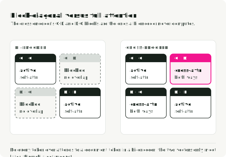
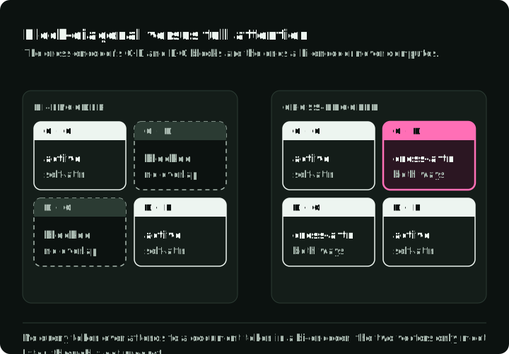
In a bi-encoder, the query is encoded before any document is seen. A cross-encoder sees the query and candidate together, so it can use their token-level relationship. This can help with cases such as:
- Negation: “headphones that are not wireless.” A pooled embedding may underweight the negation, while joint encoding gives the model a direct query-document interaction. This is a hypothesis to verify with a targeted slice, not a guarantee.
- Qualification: “laptop under $500.” Joint encoding can relate the constraint to a price in the product text, though structured price filters are safer when the field is available.
The cross-encoder input is formatted as [CLS] query tokens [SEP] document tokens [SEP]. [CLS] is a classification token whose final hidden state is fed through a linear head to produce a single relevance score. Segment embeddings distinguish query tokens from document tokens, and [SEP] marks the boundary between segments.
How cross-encoders are trained
Cross-encoders can learn from (query, document, relevance_label) examples with pointwise, pairwise, or listwise objectives. A pointwise example pairs “wireless headphones” with “Sony WH-1000XM5 Wireless Headphones” and the label 1.0.
A common classifier maps the final [CLS] representation to a score. Binary labels may use binary cross-entropy; graded relevance can use regression, ordinal, pairwise, or listwise losses. Choose with held-out ranking metrics rather than assuming one objective is universally better.
Hard negative mining also helps train cross-encoders. Cross-encoders are expensive to train — each training example needs a full forward pass through the concatenated sequence — so you can’t afford to waste compute on trivially easy negatives. The practical recipe: use a bi-encoder to retrieve the top-K candidates for each training query, then pull hard negatives from specific rank ranges (e.g., ranks 10–100). That gives the cross-encoder examples where telling relevant from irrelevant requires deep token interaction.
Reranking the retrieved candidates
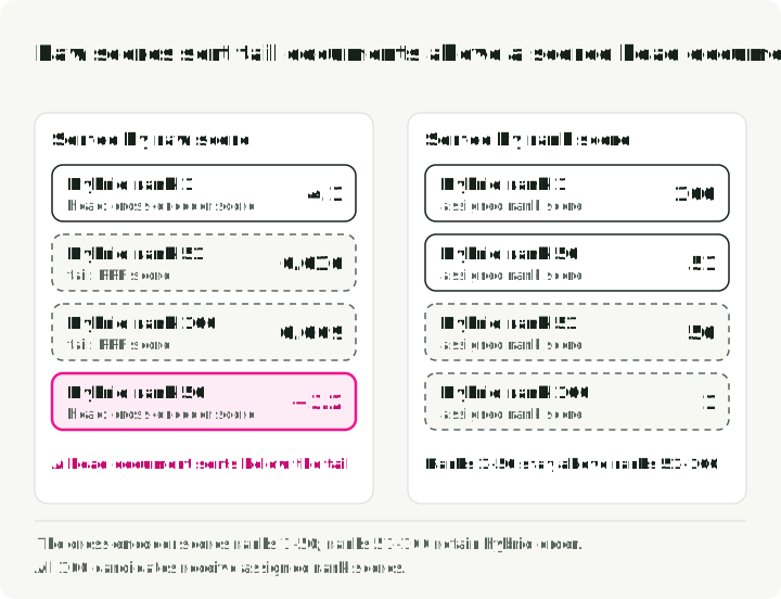
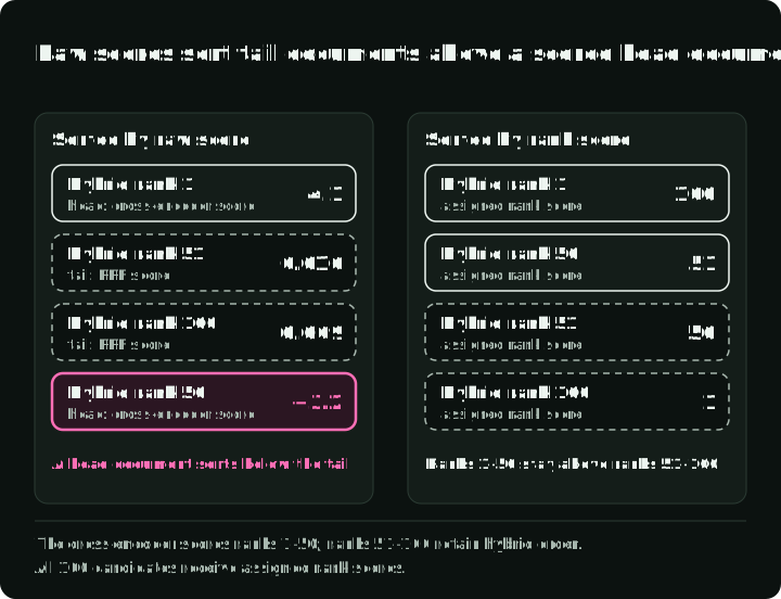
The stage sends (query, document) pairs for the first 50 hybrid candidates to CrossEncoder.predict, puts those candidates in score order, then appends the unscored candidates in their previous order. The figure sorts four of the 100 candidates both ways and shows why the merge assigns new rank scores instead of keeping the raw scores:
# From src/search_ranking_stack/stages/s04_cross_encoder.py

def rank_scores(ordered_ids):
    return {doc_id: float(len(ordered_ids) - rank) for rank, doc_id in enumerate(ordered_ids)}

def merge_head_and_tail(original, scored_head):
    """original: hybrid (doc_id, rrf_score) pairs in rank order.
    scored_head: (doc_id, cross_encoder_score) pairs for the first len(scored_head)."""
    head = sorted(scored_head, key=lambda item: (-item[1], item[0]))
    tail = original[len(scored_head) :]
    return rank_scores([doc_id for doc_id, _ in head + tail])
The full stage adds model loading, the 2,048-character document cutoff, and a check that every score is finite.
The model card shows that cross-encoder scores can be negative. Do not mix them with the RRF scores of the unscored tail: a positive RRF score can sort an unscored tail document above a negatively scored head document. Assign strictly decreasing rank scores, as rank_scores does. These are rank scores for evaluation, not calibrated relevance estimates.
The speed-quality tradeoff
Why not use cross-encoders for everything? Because you cannot pre-compute the scores. Bi-encoder document embeddings are query-independent, so you compute them once and store them. A cross-encoder’s output depends on both the query and the document together. The relevance score for “wireless headphones” paired with a Sony product comes from the joint self-attention between those specific tokens. You can cache a repeated query-document pair, but its score cannot be reused for a different query.
A bi-encoder needs one query encoding plus a vector search over pre-computed document embeddings. A cross-encoder scores every query-document pair in the shortlist, with cost that grows with both candidate count and sequence length. Batching helps, but scoring 100,000 candidates is still the wrong operating point; retrieve first and benchmark the largest shortlist that meets the quality and latency targets.
LLM listwise reranking
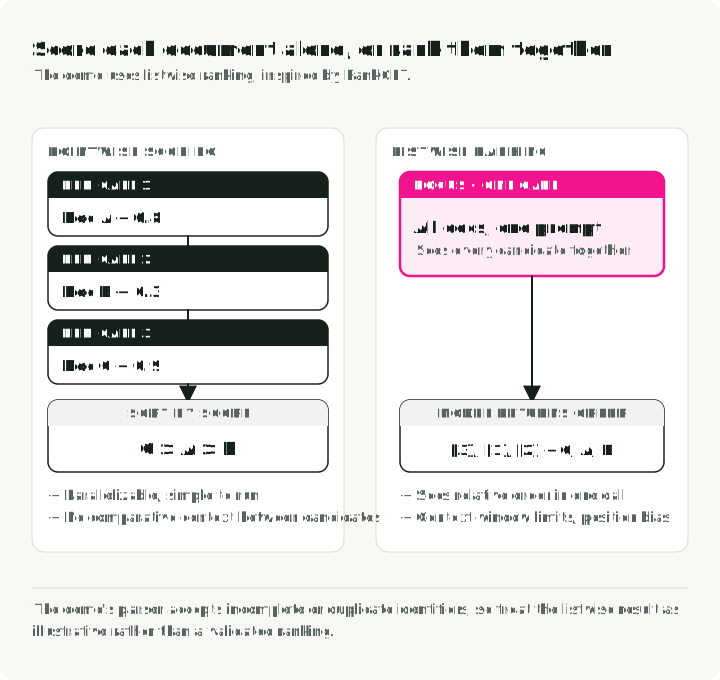
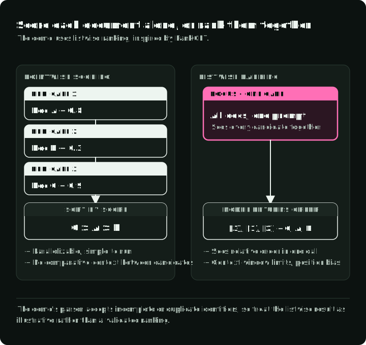
The final demo stage uses an LLM for listwise reranking. Instead of scoring each document independently, the model sees the top 10 and returns an ordering. Inspired by RankGPT, the prompt makes relative comparison explicit, but it also introduces context limits, position bias, parsing failures, and run-to-run variance.
The listwise prompt
The prompt template asks the LLM to consider the ESCI relevance hierarchy:
# src/search_ranking_stack/stages/s05_llm_rerank.py

def _create_listwise_prompt(query, documents, max_words=200):
    n = len(documents)

    doc_texts = []
    for i, (_doc_id, doc_text) in enumerate(documents, start=1):
        words = doc_text.split()[:max_words]
        doc_texts.append(f"[{i}] {' '.join(words)}")

    docs_formatted = "\n\n".join(doc_texts)

    return (
        f"I will provide you with {n} product listings, each indicated by a numerical "
        f"identifier [1] to [{n}]. Rank the products based on their relevance to the "
        f'search query: "{query}"\n\n'
        "Consider:\n"
        "- Exact matches (product satisfies all query requirements) should rank highest\n"
        "- Substitutes (functional alternatives) should rank above complements\n"
        "- Completely irrelevant products should rank lowest\n\n"
        f"{docs_formatted}\n\n"
        "Rank the products from most relevant to least relevant.\n"
        "Output ONLY a comma-separated list of product identifiers, e.g.: [3], [1], [2], ...\n"
        "Do not explain your reasoning. Only output the ranking."
    )
Three execution modes
The demo supports three backends for LLM reranking:
| Mode | Model | How it runs |
|---|---|---|
ollama | llama3.2:3b (set OLLAMA_MODEL to change it) | Local via the Ollama API |
api | Claude Haiku (set LLM_MODEL_API in config.py) | Anthropic API; uv sync --extra api first |
local | Qwen/Qwen2.5-1.5B-Instruct | HuggingFace Transformers; uv sync --extra llm first |
Parsing and fallback
The parser extracts the numbered identifiers from the model response. It accepts a ranking only if it lists every candidate exactly once:
# src/search_ranking_stack/stages/s05_llm_rerank.py

def _parse_ranking(output: str, n: int) -> list[int] | None:
    """Return 0-based positions if the output ranks IDs 1..n exactly once."""
    positions = [int(m) - 1 for m in re.findall(r"\[(\d+)\]", output)]

    # Reject missing, duplicate, and out-of-range IDs.
    if sorted(positions) != list(range(n)):
        return None

    return positions
When the parser returns None, the demo keeps the entire cross-encoder order for that query and counts a fallback. A backend error counts as a fallback too. run-all prints the fallback rate and saves it next to the metrics. For example, [3] > [1] > [3] is rejected: ID 3 is repeated and IDs 2 and 4 to 10 are missing.
Results from this ESCI sample
Results use the small_version sample described above; it is not held out. The rows come from one run of uv run run-all --llm-mode ollama with llama3.2:3b as the LLM.
| Stage | NDCG@10 | MRR | Recall@100 | NDCG Delta |
|---|---|---|---|---|
| BM25 | 0.585 | 0.812 | 0.741 | — |
| Dense Bi-Encoder | 0.611 | 0.808 | 0.825 | +0.026 |
| Hybrid (RRF) | 0.628 | 0.834 | 0.842 | +0.017 |
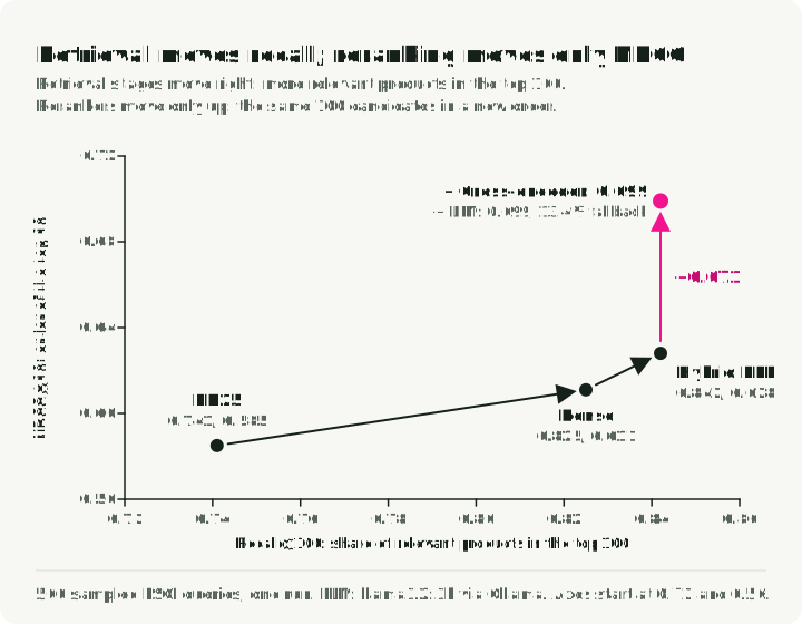
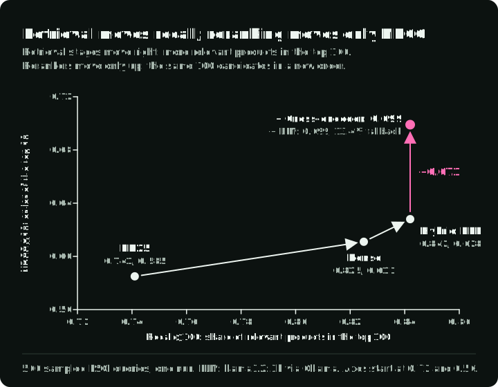
| + Cross-Encoder | 0.699 | 0.886 | 0.842 | +0.071 |
| + LLM Reranker (13.4% fallback) | 0.699 | 0.884 | 0.842 | +0.000 |
The chart plots each row’s Recall@100 against its NDCG@10:
What the recorded results support
Hybrid search beats either method on its own. Hybrid RRF reaches NDCG@10 0.628, above BM25 (0.585) and Dense (0.611). It also has the highest Recall@100 of the three retrieval rows (0.842). The two methods can fail on different queries, and fusion recovers documents that either one alone misses.
The cross-encoder gives the largest gain. It raises NDCG@10 from 0.628 to 0.699 and MRR from 0.834 to 0.886 while scoring only 50 candidates per query. In the top 10, the share of Exact products rises from 36.0% (hybrid) to 41.4%.
Recall is set at retrieval in this demo. Both rerankers retain all 100 hybrid candidates, so Recall@100 stays at 0.842. To raise it, change which 100 candidates retrieval returns.
A small local LLM adds nothing on this sample. llama3.2:3b leaves NDCG@10 at 0.699 and lowers MRR slightly. 67 of 500 answers (13.4%) failed the parser and kept the cross-encoder order, so the LLM order was applied on 433 queries. A larger model or the API mode may behave differently; measure it the same way, with the fallback rate next to the score.
Dense retrieval beats BM25 on this sample. Inspect query slices before assigning the cause. Vocabulary mismatch is one plausible driver, but the sample construction, tokenizer, model training domain, and corpus fields also affect the comparison.
Indexing dense vectors beyond the demo
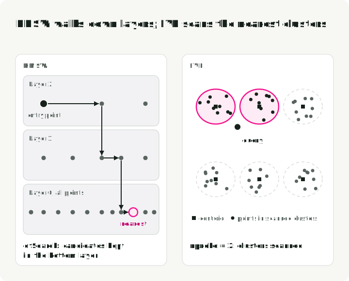
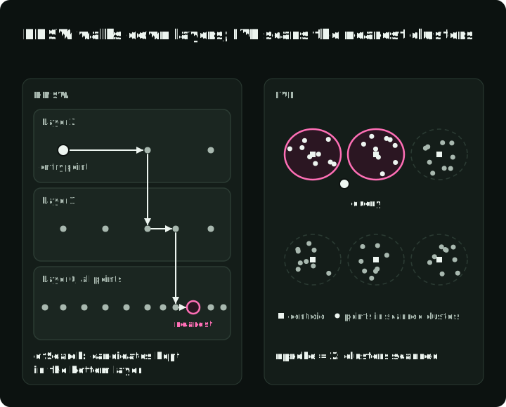
Dense embeddings only become useful at scale once you have an Approximate Nearest Neighbor (ANN) index. The demo uses brute-force cosine similarity (which is fine at 9,870 documents), but production systems need specialized indexes. The two common families search in different ways, and each has one search-time setting that trades recall for query work. The figure shows the path HNSW follows and the clusters IVF scans:
HNSW (hierarchical navigable small world)
HNSW builds a multi-layer graph: sparse upper layers navigate broadly, and denser lower layers refine the neighborhood. M controls graph connectivity, while efSearch trades query work for recall. Useful values depend on dimension, distance distribution, filters, implementation, and target recall.
Graph indexes can lose recall under heavy updates or restrictive filters; one Qdrant issue shows filtered recall recovering only after a rebuild. Test your update and filter pattern, including rebuild time.
IVF (inverted file)
IVF indexes partition vector space into clusters, then scan the nprobe clusters closest to the query. They can offer a useful memory, build-time, and recall trade-off, especially when combined with compression. Update semantics and performance depend on the implementation rather than the index family alone.
RaBitQ (Gao & Long, SIGMOD 2024) is a randomized quantizer that can be combined with IVF. It normalizes centered vectors, uses a random orthogonal rotation, and encodes signs with one bit per dimension. Distance estimation also uses correction factors and vector norms; the paper’s error bounds apply to that estimator and its assumptions. Use it when memory is the limit and the quantized distance estimates still meet your recall target.
| Dimension | HNSW graph | IVF clusters |
|---|---|---|
| Query control | efSearch | nprobe |
| Build control | Connectivity and construction beam | Cluster count and training sample |
| Memory profile | Graph edges plus vectors | Centroids, lists, and stored vectors |
| Update behavior | Database-specific repair/cleanup | Database-specific list maintenance |
| Usually chosen when | Vectors fit in RAM and you need low latency at high recall | Memory or corpus size is the limit; pair with PQ or RaBitQ |
For either index, measure the recall-latency-memory curve on your own data and query load.
Uber cut latency and CPU by lowering a per-shard candidate count with little recall loss; tune that count on production-like traffic.
Optional extensions after the core pipeline
Once retrieval and reranking have separate measurements, several extensions become easier to evaluate without obscuring the core pipeline.
Query understanding
Query expansion and rewriting can address vocabulary mismatch before retrieval. Query2doc generated pseudo-documents and reported BM25 gains on its MS MARCO experiments. Expansion can also introduce the wrong intent, so compare recall and precision on ambiguous, navigational, and exact-identifier query slices.
Practical patterns: abbreviation expansion, entity enrichment, sub-query decomposition for multi-hop reasoning, and RAG-Fusion — generating multiple query variants and combining results via RRF.
LLM-assisted relevance labeling
LLMs can draft relevance labels when human judgments are scarce. Pinterest’s relevance-labeling work describes expanding training data beyond human labels and distilling an LLM-based relevance model for serving. An LLM label is still model output: calibrate it against blinded human judgments, inspect disagreement slices, and keep a human gold set for regression tests.
Useful controls include:
- a rubric with concrete relevance boundaries and examples;
- blinded human calibration and periodic rechecks;
- order randomization and repeated judgments for unstable cases;
- model panels where their added cost improves agreement; and
- explicit checks for position and central-tendency bias.
Knowledge distillation
When an LLM teacher adds value but cannot meet serving constraints, distillation is one option:
- Use a powerful LLM (the teacher) to rerank thousands of training queries offline; only the small student runs per request
- Train a small, fast cross-encoder (the student, ~100M–200M parameters) to mimic the LLM’s ranking distribution
- Compare the student with both teacher and baseline on quality, calibration, and serving cost
InRanker distills MonoT5-3B into 60M and 220M parameter models, respectively 50x and about 13x smaller, with improved out-of-domain effectiveness over their undistilled versions. The Rank-Without-GPT approach produces 7B open-source listwise rerankers that reach 97% of the compared GPT-4 reranker’s effectiveness by nDCG@10 on TREC-DL-19 and TREC-DL-20, using QLoRA fine-tuning.
Published compression results are starting points, not expected production ratios. Distillation can inherit the teacher’s biases and may lose quality on rare query slices, so keep the original relevance judgments in the evaluation loop.
Personalization and position bias
A search for “apple” should return iPhones for a tech enthusiast and apple recipes for someone who’s been browsing cooking content.
A common retrieval architecture for personalization uses a two-tower embedding model: the query tower encodes the query and user context, while the item tower encodes items and metadata. The figure shows which side runs per request, which side is computed offline, and where the “apple” query lands for two users:
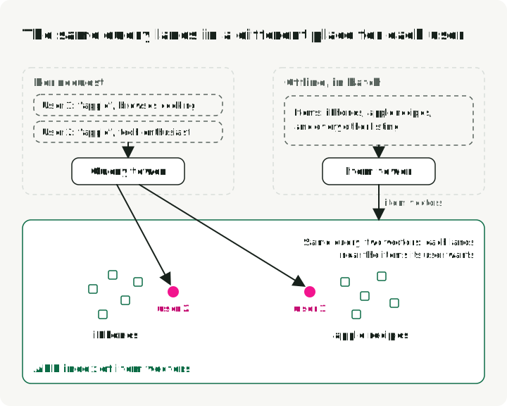
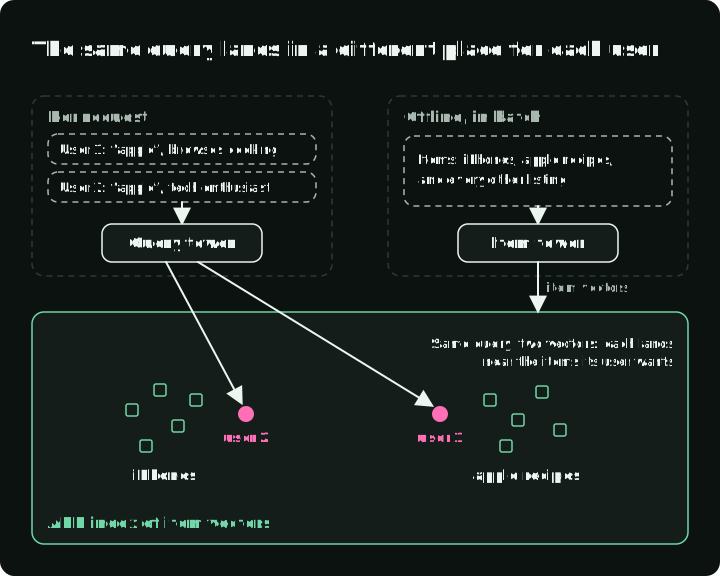
The offline/online split supports approximate-nearest-neighbor retrieval; its latency still depends on the encoder, index, filters, and serving system. Three production designs use learned embeddings in different places. Airbnb learns listing embeddings from users’ click sessions and uses similarity to recently clicked listings as search-ranking features. Pinterest’s OmniSearchSage learns one query embedding together with pin and product embeddings. Uber uses a two-tower model to retrieve a few hundred stores for the Uber Eats home feed.
Click data carries position and exposure bias. PAL is one debiasing approach: jointly train an exposure module and a click-given-exposure module, then serve the latter without a position input. It is not a universal fix; randomized interventions, inverse-propensity methods, and counterfactual evaluation may be more appropriate for another product.
Domain adaptation with synthetic queries
A common search-strategy mistake is assuming a model trained on general web data (like MS MARCO) will work well on a specialized domain. This is the out-of-domain (OOD) problem.
Synthetic query generation can reduce the labeled-data bottleneck. InPars generates queries for documents and filters pairs for training. Generative Pseudo-Labeling (GPL) adds a teacher-labeling step:
- Generate queries from the target document corpus.
- Retrieve negative documents for each generated query.
- Use a cross-encoder teacher to score positive and negative pairs, producing a relevance-score margin.
- Train the dense retriever to match those margins.
Synthetic pairs can help when real queries are scarce, but they reflect the generator and prompt. Deduplicate them, filter implausible queries, and validate on real held-out traffic.
An experiment sequence
Add complexity only when the previous stage exposes a measured failure. Each step names the failure that justifies it:
- Establish a baseline. Run BM25 or the current lexical system against a judged query set. Record recall, NDCG, latency, and the query groups where it fails.
- Recover missing candidates. Test dense retrieval and fusion when the baseline misses relevant documents. Tune the candidate cutoff against recall and cost.
- Improve the order. Add a cross-encoder when relevant candidates are present but ranked too low. Choose its shortlist size by measuring quality and latency at several cutoffs. In the demo, this step raised NDCG@10 from 0.628 to 0.699.
- Adapt to the domain. Fine-tune or distill after generic models show stable domain-specific failures. Keep real held-out judgments separate from synthetic training data.
- Test expensive reranking. Try listwise or reasoning-based reranking only when the added quality survives repeated runs and justifies its latency, cost, privacy requirements, and fallback complexity. In the demo,
llama3.2:3bdid not pass this test.
The starting stack and the judgments to collect depend on the product:
| Use case | Candidate starting stack | Validate |
|---|---|---|
| Product search | BM25 + dense retrieval + RRF + cross-encoder | Attribute recall, substitutions, latency, business constraints |
| Documentation search | Hybrid retrieval + cross-encoder | Exact identifiers, semantic questions, version filters |
| Support deflection | Hybrid retrieval + citation checks | Retrieval recall, grounding, abstention |
| Marketplace or listings | Lexical filters + dense retrieval + business reranker | Availability, freshness, policy, seller diversity |
| Small internal corpus | BM25 baseline, then a reranker | Whether vocabulary mismatch justifies a dense index |
| High-stakes legal or medical search | Recall-focused retrieval plus expert review | Coverage, provenance, calibrated abstention |
For every comparison, keep a real held-out judgment set separate from training data. Record per-query rankings, failures, latency, and cost so an aggregate gain can be traced back to the changed stage. Expensive layers also need explicit privacy and fallback policies.
Research directions to evaluate separately
Reasoning rerankers and search-using agents are promising, but they answer different questions from the five-stage product-search demo.
Reasoning-based rerankers
Rank1 trains rerankers with reasoning traces and reports strong results on the BRIGHT benchmark. That evidence is relevant to reasoning-heavy retrieval, not a direct prediction for ESCI product search.
For legal or scientific search, compare reasoning rerankers with strong cross-encoder and listwise baselines on expert judgments, citations, latency, and failure consistency.
Agentic search
Search-o1 studies a model that issues additional searches during multi-hop question answering. This is an orchestration problem — query generation, stopping, evidence use, and answer evaluation — not another reranking stage. Evaluate it with end-task correctness and citation support, not only retrieval metrics.
References
Papers
- Reciprocal Rank Fusion — Cormack et al., 2009
- RankGPT: LLMs as Zero-Shot Listwise Rerankers — Sun et al., EMNLP 2023 Outstanding Paper
- Rank1: Reasoning-Based Reranking — Weller et al., COLM 2025
- Query2doc: LLM Query Expansion — Wang et al., EMNLP 2023
- GPL: Generative Pseudo Labeling — Domain adaptation for dense retrieval
- InRanker: Distilled Reranker — 50x size reduction with competitive performance
- Search-o1: Agentic Retrieval — Li et al., 2025
- BEIR Benchmark — Thakur et al., NeurIPS 2021
- Sentence-BERT — Reimers & Gurevych, EMNLP 2019
- InfoNCE / CPC — van den Oord et al., 2018
- SimANS: Hard Negative Sampling — Zhou et al., EMNLP 2022
- Passage Reranking with BERT — Nogueira & Cho, 2019
- HNSW — Malkov & Yashunin, 2016
- DiskANN — Subramanya et al., NeurIPS 2019
- RaBitQ — Gao & Long, SIGMOD 2024
- Replacing Judges with Juries — Verga et al., 2024
- RAG-Fusion — Rackauckas, 2024
- InPars — Bonifacio et al., SIGIR 2022
- BRIGHT Benchmark — Su et al., ICLR 2025
- Rank-without-GPT — Zhang et al., ECIR 2025
- Pinterest LLM Search Relevance — Wang et al., 2024
- OmniSearchSage — Agarwal et al., WWW 2024
- PAL: Position-bias Aware Learning — Guo et al., RecSys 2019
Datasets and benchmarks
- Amazon ESCI: Shopping Queries Dataset — KDD Cup 2022
- BEIR: Benchmarking IR — Heterogeneous benchmark for zero-shot evaluation
- MTEB: Massive Text Embedding Benchmark — Embedding model leaderboard
- ESCI Paper — Reddy et al., 2022
Models used in the demo
- all-MiniLM-L6-v2 — 22M parameter bi-encoder
- ms-marco-MiniLM-L12-v2 — 33M parameter cross-encoder
- Sentence-Transformers — Neural retrieval model framework
Tools and platforms
- rank_bm25 — BM25 implementation in Python
- Pyserini BEIR Reproductions — Lucene BM25 baselines for BEIR
- pytrec_eval — TREC evaluation toolkit
- Elasticsearch — Hybrid search with Retrievers API
- Vespa — Unified search and recommendation engine
- Weaviate — Vector database with hybrid search
- Qdrant — Vector database with multi-stage queries
Industry references
- Airbnb Listing Embeddings — Grbovic & Cheng, KDD 2018
- Uber Delivery Search — Uber Engineering, 2025
- Uber Two-Tower Embeddings — Uber Engineering, 2023
- Elastic Rerank — Elastic, 2024
Demo project
- search-ranking-stack — Working demo of the pipeline in this post