Reading the Math in AI Papers · Part 3 of 3

Reading training objectives: distillation, DPO and GRPO

Viacheslav Dubrov

2026-11-12 · Updated 2026-11-12 · 14 min · Model Engineering

Distillation, Direct Preference Optimization (DPO) and Group Relative Policy Optimization (GRPO) all change a language model’s probabilities, but they use different training examples and feedback. This guide is for engineers who want to understand those differences before reading the full objectives. The diagrams show where feedback comes from and how it changes probability comparisons; the equations give the corresponding operations.

In ordinary supervised fine-tuning, the model learns to predict the next token in saved examples. The methods below change the feedback: a teacher supplies probabilities, a preference pair says which answer is better, or a reward scores answers sampled during training. A policy is simply the model that generates answers. All logarithms below are natural logs.

Part 1 explains how to read an equation and provides a notation reference. Here, each section explains the terms it needs and can be read on its own.

Classical distillation: a temperature on both softmaxes

A training label names the correct outcome: for next-token prediction, it is the next token in a saved example. A teacher model supplies more information: its probabilities for every candidate token, including plausible alternatives. Distillation trains a smaller student to match those probabilities. Training reduces a numerical loss by changing the student’s parameters; the teacher’s stay fixed.

Hinton et al.’s distillation paper, §2, softens both models’ probabilities before comparing them. Divide each logit—the raw score before softmax—by a temperature $T$ :

q_i=\frac{\exp(z_i/T)}{\sum_j\exp(z_j/T)}.

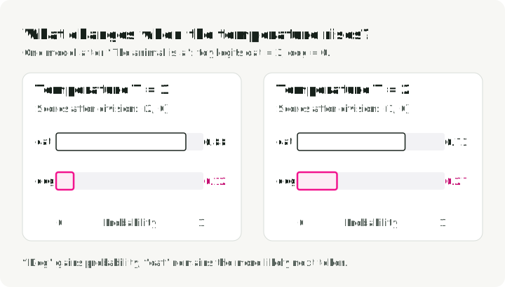
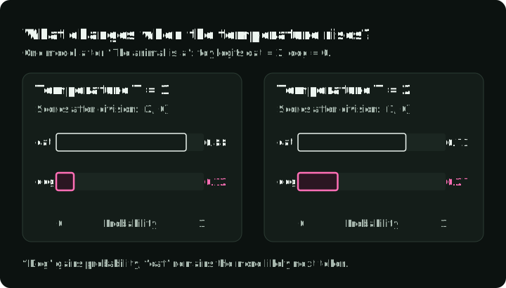
Here $z_i$ is candidate $i$ ‘s score and $q_i$ its probability. Suppose a toy model has only two possible next tokens, “cat” and “dog”, and assigns them scores $(2,0)$ after reading “The animal is a”. At $T=1$ , the probabilities are about $(0.88,0.12)$ ; at $T=2$ , they become $(0.73,0.27)$ . The smaller score now contributes more to the comparison. Both teacher and student use the same temperature.

The bars show how the same two scores become a less concentrated distribution as temperature rises.

$For the toy next tokens cat and dog, logits 2 and 0 give probabilities 0.88 and 0.12 at temperature 1, and 0.73 and 0.27 at temperature 2. Both charts use the same zero-to-one scale. Dog gains probability.$ $For the toy next tokens cat and dog, logits 2 and 0 give probabilities 0.88 and 0.12 at temperature 1, and 0.73 and 0.27 at temperature 2. Both charts use the same zero-to-one scale. Dog gains probability.$

The training loss combines the ordinary label loss with a loss for matching the softened teacher distribution. Write $p^{(T)}$ for the teacher’s probabilities and $q^{(T)}$ for the student’s at temperature $T$ . For one labeled input:

\begin{aligned} \mathcal L&=(1-\lambda)\bigl(-\log q_y^{(1)}\bigr)\\ &\quad+\lambda T^2 D_{\mathrm{KL}}\bigl(p^{(T)}\Vert q^{(T)}\bigr). \end{aligned}

Here $\mathcal L$ is the loss, $y$ is the correct next token, and $\lambda\in[0,1]$ sets the mixture. Parenthesized superscripts name temperatures, not powers. Read the first term as “penalize low probability for the correct token at $T=1$ ”. Read the second as “match the teacher’s softened probabilities”. Training averages these losses over the saved inputs and changes only the student.

$D_{\mathrm{KL}}(p\Vert q)$ is KL divergence from teacher $p$ to student $q$ . It measures how two probability distributions differ: zero when they match. The first distribution supplies the weights in the comparison, so teacher-likely outcomes receive more weight. Hinton et al. describe a cross-entropy matching term; this KL form subtracts a teacher-only constant and gives the same student gradients.

The $T^2$ factor compensates approximately for smaller gradients at higher temperatures. This is a training setting; the deployed student normally returns to $T=1$ for this softmax.

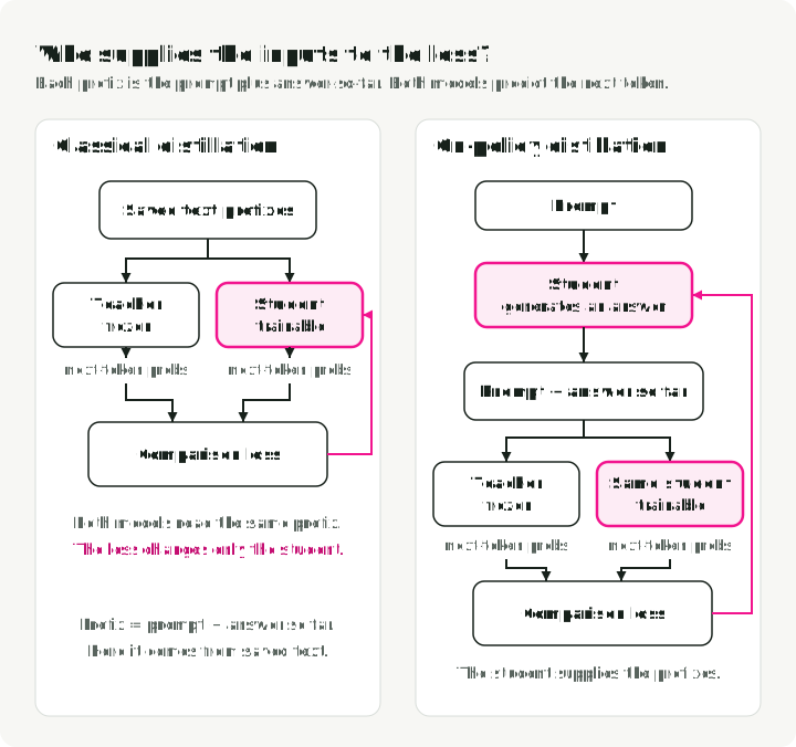
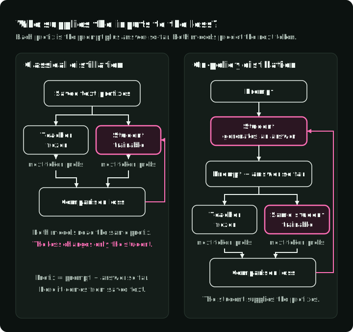
A prefix is the text already available before the next token: the prompt plus any answer tokens so far. For example, “The animal is a” is the prefix before “cat”. In the figure, both models read the same prefix and produce next-token probabilities. On the left, prefixes come from saved examples. On the right, they come from answers the student generates during training. Both paths use the comparison loss to update only the student.

$Classical distillation sends fixed inputs to a frozen teacher and a trainable student, then compares their probabilities. On-policy distillation first samples text from the student; teacher and student then compare next-token probabilities on prefixes of that text. Only the student is updated.$ $Classical distillation sends fixed inputs to a frozen teacher and a trainable student, then compares their probabilities. On-policy distillation first samples text from the student; teacher and student then compare next-token probabilities on prefixes of that text. Only the student is updated.$

There is also distillation without probability matching. DeepSeek-R1’s distilled models, §2.4, were fine-tuned on 800,000 samples curated with DeepSeek-R1 beforehand. They used a supervised loss on saved text; a teacher did not have to run during that training.

The detailed distillation reading explains the mixed loss and temperature scaling.

On-policy distillation: the student comes first in the KL

A student generating its own answer can reach prefixes—prompt plus answer-so-far—that never occurred in the training dataset. On-policy distillation obtains feedback on text the student actually produces. Given a prompt, the student samples an answer. A frozen teacher then evaluates the same prefixes, so training compares the two models where the student needs guidance.

On-policy describes that source of training text. It does not, by itself, prescribe a particular loss. The examples here use reverse KL, with the student first:

D_{\mathrm{KL}}(q_\theta\Vert p) =\mathbb E_{y\sim q_\theta}\left[\log\frac{q_\theta(y\mid x)}{p(y\mid x)}\right].

For a fixed prompt $x$ , $q_\theta$ is the student with trainable parameters $\theta$ , $p$ the teacher, and $y$ an answer sampled from the student. The expression compares the probability the student assigned to its answer with the teacher’s probability. Averaged over student answers, it penalizes the student for giving high probability to text the teacher considers unlikely.

This differs from asking the student to cover every outcome the teacher might produce. When a small student cannot match the teacher’s full distribution, reverse KL can favor concentrating on some of the teacher’s likely outputs. MiniLLM, §2.1, equation (1), uses this objective. Its actual training procedure also mixes teacher samples into generation and adjusts the gradient to reduce variance and length bias; the diagram shows the basic on-policy setup, not all of MiniLLM’s modifications.

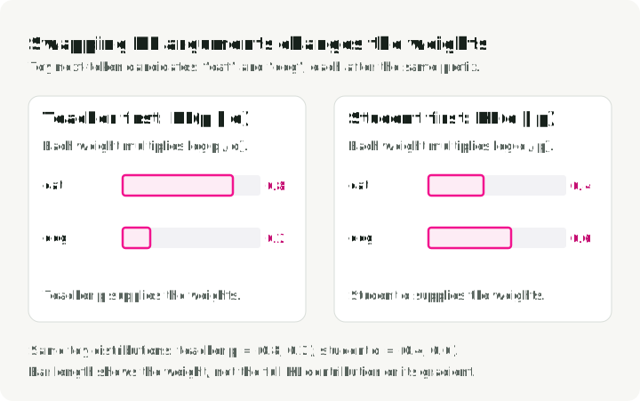
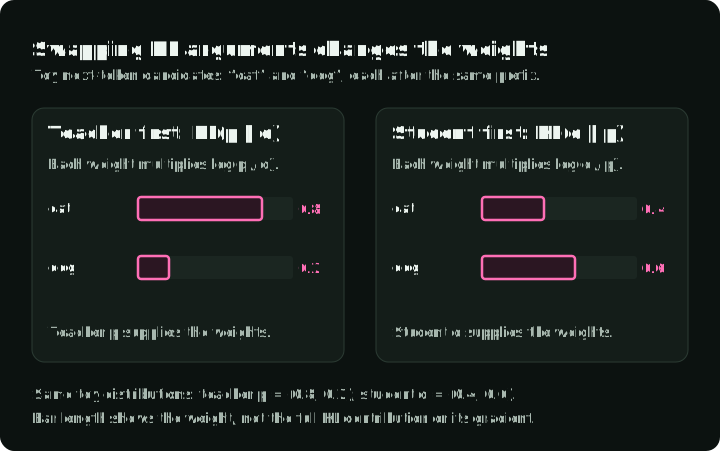
In the toy example below, teacher and student assign different probabilities to “cat” and “dog” after the same prefix. KL multiplies each token’s log-ratio by its weight, then adds the two terms. Changing the first argument shifts the larger weight from “cat” to “dog”. The bars show the weights, not the complete loss contributions.

$After the same prefix, teacher probabilities for cat and dog are 0.8 and 0.2; student probabilities are 0.4 and 0.6. Forward KL weights log teacher-to-student ratios by 0.8 and 0.2. Reverse KL weights log student-to-teacher ratios by 0.4 and 0.6.$ $After the same prefix, teacher probabilities for cat and dog are 0.8 and 0.2; student probabilities are 0.4 and 0.6. Forward KL weights log teacher-to-student ratios by 0.8 and 0.2. Reverse KL weights log student-to-teacher ratios by 0.4 and 0.6.$

From sequence KL to token KL

An answer’s probability is built from its next-token probabilities. At each prefix of a student answer, both models predict the next token. Their differences can therefore be compared position by position, then accumulated over the answer. DeepSeek-V4, §5.1.2, equation (29), uses reverse-KL distillation from several specialist teacher models into one student. These teachers are separate models, not the expert sub-networks inside a mixture-of-experts layer.

At position $t$ , let $q_t(v)=q_\theta(v\mid x,y_{<t})$ be the student’s probability for candidate token $v$ . The prefix contains prompt $x$ and the preceding answer tokens $y_{<t}$ ; $p_t(v)$ is the teacher’s probability at that same prefix. Then:

\begin{aligned} d_t&=\sum_{v\in V}q_t(v)\log\frac{q_t(v)}{p_t(v)},\\ D_{\mathrm{KL}}(q_\theta\Vert p) &=\mathbb E_{y\sim q_\theta}\left[\sum_t d_t\right]. \end{aligned}

$V$ is the vocabulary and $d_t$ the next-token KL at one prefix. Read the inner sum as “compare every candidate token, weighted by the student’s probability”. Sum these comparisons over positions, then average over answers the student generates. The outer expectation still samples text, even when each $d_t$ sums the whole vocabulary.

One sampled token or the full vocabulary

The teacher can score just the token the student chose, or return probabilities for the entire vocabulary. The first option transfers less information; the second compares all possible next tokens at that prefix. DeepSeek-V4 reports unstable training with its one-token estimate and uses the full-vocabulary comparison. This makes the token comparison exact at a given prefix; the prefixes still come from sampled answers.

Both models read “The animal is a” and return the probabilities shown below. The highlighted rows enter the loss used to update the student. The full-vocabulary version includes “dog” and “fox” even though the student chose “cat”; the one-token version estimates that comparison from the chosen token alone.

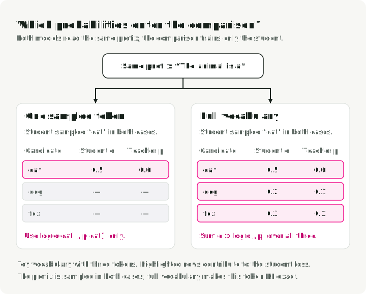
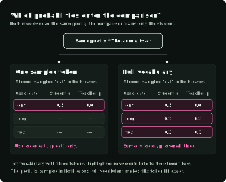
$At the prefix “The animal is a”, the student samples cat. A one-token estimate compares probabilities for cat only. Full-vocabulary KL includes cat, dog and fox in this toy vocabulary, weighting each log-ratio by the student probability. The prefix remains sampled.$ $At the prefix “The animal is a”, the student samples cat. A one-token estimate compares probabilities for cat only. Full-vocabulary KL includes cat, dog and fox in this toy vocabulary, weighting each log-ratio by the student probability. The prefix remains sampled.$

Using the three rows, $d_t=0.5\log(0.5/0.6)+0.2\log(0.2/0.3)+0.3\log(0.3/0.1)\approx0.157$ . The sampled “cat” log-ratio alone is about $-0.182$ . One sample can be negative even though the full KL is nonnegative.

The detailed on-policy reading covers the sequence-to-token derivation, sampling corrections and gradient estimates.

DPO: a logistic loss on two log-ratios

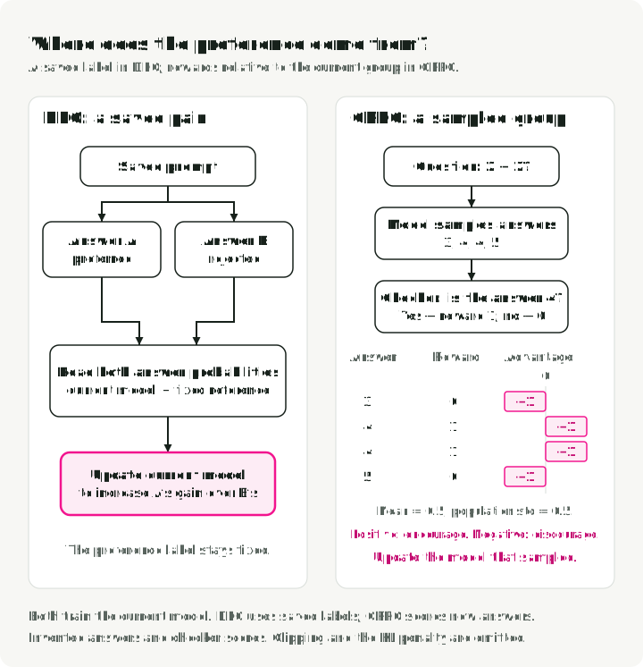
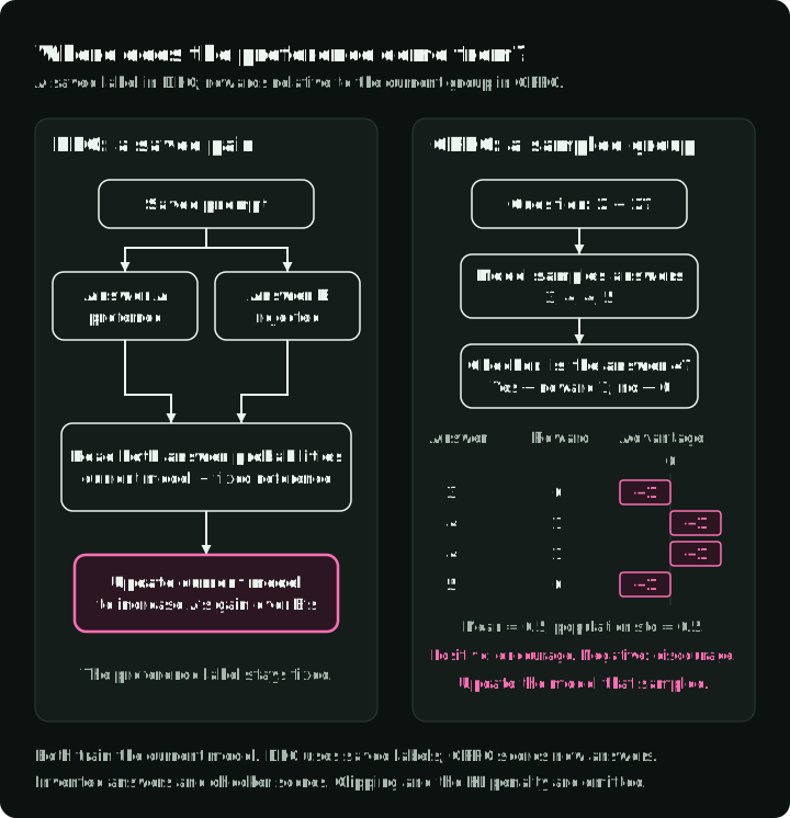
DPO starts with a saved preference pair: one prompt, a preferred answer and a rejected answer. The pair might come from human judgments on earlier model outputs. During training, the model reads each saved answer token by token and records its probability given the prompt and preceding tokens. Adding those log-probabilities gives the answer’s log-probability. This scores how likely the text is under the model; the saved preference label says which answer is better.

In a conventional RLHF procedure, preference pairs first train a separate reward model, and reinforcement learning then trains the language model against that reward. DPO, §4, equation (7), instead trains the language model directly from the pairs. A frozen reference model scores those same answers for comparison. Training changes only the current model; neither model needs to generate new answers for this step.

For each answer, subtract its reference log-probability from its current log-probability. Call this change its gain. DPO compares the preferred answer’s gain with the rejected answer’s gain:

\begin{aligned} g(y)&=\log\frac{\pi_\theta(y\mid x)}{\pi_{\mathrm{ref}}(y\mid x)},\\ \Delta&=g(y_w)-g(y_l),\\ \mathcal L_{\mathrm{DPO}} &=\mathbb E_{(x,y_w,y_l)\sim\mathcal D} \bigl[-\log\sigma(\beta\Delta)\bigr]. \end{aligned}

Here $x$ is the prompt, $y_w$ and $y_l$ are its preferred and rejected answers, and $\pi_\theta$ and $\pi_{\mathrm{ref}}$ are the current and reference models. The sigmoid $\sigma$ maps a number into $(0,1)$ , and $\beta$ is a positive scale. Read the final line as “average the bracketed pair loss over saved pairs in dataset $\mathcal D$ ”. Increasing $\Delta$ lowers that loss; training minimizes $\mathcal L_{\mathrm{DPO}}$ by changing the current model’s parameters $\theta$ .

For example, if the preferred answer gains 2 in log-probability and the rejected answer loses 1, then $\Delta=2-(-1)=3$ . The preference has moved in the intended direction relative to the reference. The loss has no separate KL term and does not enforce a maximum distance from the reference.

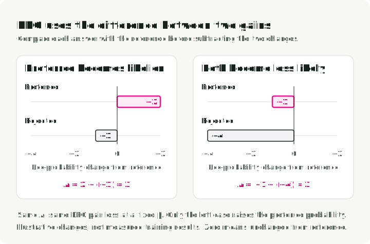
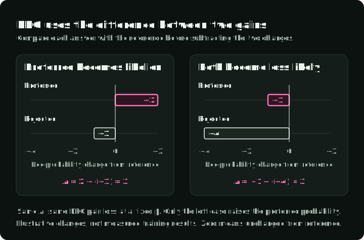
The difference alone can hide a problem: the preferred answer can become less likely while the rejected answer becomes less likely even faster. The loss still improves. Smaug studies this failure, so inspect the individual answer probabilities as well as the preference loss.

The two cases below give the same $\Delta=3$ and therefore the same pair loss at a fixed $\beta$ . Only the left case makes the preferred answer more likely than it was under the reference.

$Two cases share a log-probability-change axis. Preferred plus 2 and rejected minus 1 give a gain difference of 3. Preferred minus 1 and rejected minus 4 also give 3, although both answer probabilities declined from the reference.$ $Two cases share a log-probability-change axis. Preferred plus 2 and rejected minus 1 give a gain difference of 3. Preferred minus 1 and rejected minus 4 also give 3, although both answer probabilities declined from the reference.$

In the next figure, DPO’s feedback is attached to a saved pair. GRPO generates four answers to “2 + 2?” during training. An answer checker gives 1 for “4” and 0 otherwise. Comparing each reward with the group’s average produces an advantage: positive feedback encourages the sampled answer’s tokens, and negative feedback discourages them. The next section shows that calculation and the limits on its effect.

$DPO uses current and frozen reference models to score two saved answers, then updates the current model. GRPO samples 3, 4, 4 and 5 for the question 2 plus 2. A checker assigns rewards 0, 1, 1 and 0. Group-relative advantages of minus 1, plus 1, plus 1 and minus 1 guide updates to the current model.$ $DPO uses current and frozen reference models to score two saved answers, then updates the current model. GRPO samples 3, 4, 4 and 5 for the question 2 plus 2. A checker assigns rewards 0, 1, 1 and 0. Group-relative advantages of minus 1, plus 1, plus 1 and minus 1 guide updates to the current model.$

The detailed DPO reading derives the loss from the reward-regularized objective and works through its gradient.

GRPO: PPO’s objective with a group baseline

Group Relative Policy Optimization samples several answers to the same question, scores them, and compares each score with the group’s average. A correct answer among mostly incorrect answers receives positive feedback; an incorrect answer among correct ones receives negative feedback. For math or code, scoring can use an answer checker or tests. Other tasks can use a reward model.

DeepSeekMath, §4.1.1, introduced GRPO as a variant of Proximal Policy Optimization (PPO). DeepSeek-R1, §2.2.1, later used it. The central change is how it computes the advantage, the relative reward that guides the update:

A_i=\frac{r_i-\operatorname{mean}(r_1,\ldots,r_G)}{\operatorname{std}(r_1,\ldots,r_G)}.

$r_i$ is answer $i$ ‘s reward and $G$ is the number of answers to one question. Subtracting the mean tells us which answers scored above or below the group. Dividing by the standard deviation scales those differences. In the illustrated group $(0,1,1,0)$ , the mean is $0.5$ and the population standard deviation is $0.5$ , giving advantages $(-1,1,1,-1)$ .

What changes from PPO

PPO commonly trains a separate value model to estimate future reward from a partial answer. GRPO uses the group’s scores as its baseline instead, so it does not train that value model. It still needs reward feedback, and its original objective still uses a reference model for a KL penalty. Removing the value model does not remove those other roles.

The comparison below locates the replaced value model. Its lower row shows two other inputs to training. The old or sampling model is the version that generated this batch of answers; its recorded token probabilities stay fixed while the current model trains on that batch. A separate reference model, also held fixed during these updates, supplies probabilities for the KL comparison. Both comparisons score the same token after the same prefix.

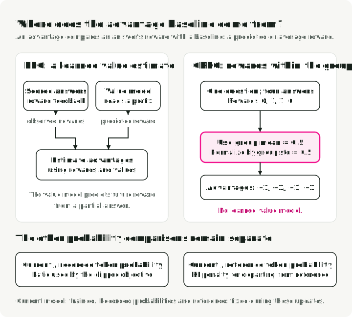
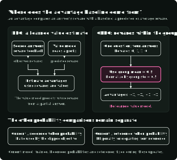
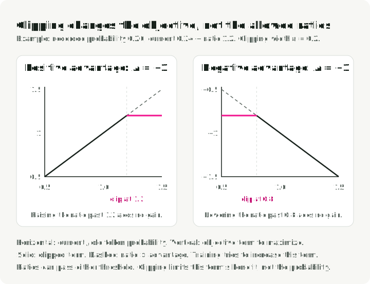
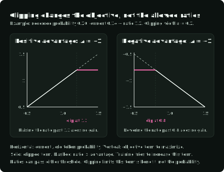
$PPO uses reward feedback and a trained value model to estimate advantages. GRPO instead normalizes each answer reward against rewards from the same question. The current-versus-sampling probability ratio and current-versus-reference KL serve separate roles in training.$ $PPO uses reward feedback and a trained value model to estimate advantages. GRPO instead normalizes each answer reward against rewards from the same question. The current-versus-sampling probability ratio and current-versus-reference KL serve separate roles in training.$

GRPO retains PPO’s clipped probability-ratio objective. If a sampled token had probability $0.20$ and the current model now assigns it $0.24$ at the same prefix, the ratio is $0.24/0.20=1.2$ . The objective weights this ratio by the answer’s advantage. Training changes the current model to increase this objective, with a separate KL penalty discouraging departure from the reference.

For one sampled answer, write $s_t$ for the prompt plus answer tokens before position $t$ , and $y_t$ for the token at that position. The part of DeepSeekMath’s equation (3) shown in the graph is:

\begin{aligned} \rho_t&=\frac{\pi_\theta(y_t\mid s_t)}{\pi_{\mathrm{old}}(y_t\mid s_t)},\\ C_t&=\min\!\bigl(\rho_t A,\\ &\qquad\operatorname{clip}(\rho_t,1-\varepsilon,1+\varepsilon)A\bigr). \end{aligned}

$\pi_\theta$ is the current model, $\pi_{\mathrm{old}}$ the sampling copy, and $A$ this answer’s group advantage. The width $\varepsilon$ sets the clipping interval. Read $\operatorname{clip}$ as “replace an out-of-range ratio with the nearest endpoint”, then $\min$ as “take the smaller of the two advantage-weighted terms”. $C_t$ is a contribution to maximize. GRPO subtracts its KL penalty and averages over tokens within answers, answers within groups, and sampled questions.

With $A=1$ , $\varepsilon=0.2$ and $\rho_t=1.5$ , the two terms are $1.5$ and $1.2$ , so $C_t=1.2$ . With $A=-1$ and $\rho_t=0.5$ , they are $-0.5$ and $-0.8$ , so $C_t=-0.8$ . These are the two flat portions of the graph.

The graph isolates one token’s contribution while holding its advantage fixed. A positive advantage favors a higher ratio; a negative advantage favors a lower one. Clipping makes the line flat where a favorable change stops improving this term. It does not impose a hard limit on the model’s actual probabilities.

$For clipping width 0.2 and advantage plus 1, the clipped objective rises with the ratio until 1.2 and then stays flat. For advantage minus 1, it stays flat below 0.8 and falls as the ratio rises above 0.8. The actual probability ratio can go beyond either threshold.$ $For clipping width 0.2 and advantage plus 1, the clipped objective rises with the ratio until 1.2 and then stays flat. For advantage minus 1, it stays flat below 0.8 and falls as the ratio rises above 0.8. The actual probability ratio can go beyond either threshold.$

The sampling copy and the reference can start with the same weights, but they serve different comparisons. The sampling copy is refreshed when collecting a new batch; its recorded probabilities remain the denominator for updates on that batch.

If every answer earns the same reward, there is no relative preference to learn. The advantage formula then divides zero by zero. Implementations need a rule for this case, such as producing zero advantages; DAPO, §3.2, instead excludes these groups and samples replacements.

The detailed GRPO reading covers the full objective, clipping cases, gradients, the sampled KL estimator, and the effect of averaging per answer or per token.

Optional equation walkthroughs

The linked detailed readings include derivations and small-number checks. They were produced with the coding-agent skills in paper-math-skills and are collected in paper-math-readings.

Sources and versions

Hinton et al. Distilling the Knowledge in a Neural Network, §2, equation (1).
Gu et al. MiniLLM, §2.1–2.2.
DeepSeek-AI. DeepSeek-V4, §5.1.2, equation (29).
Rafailov et al. Direct Preference Optimization, §4, equation (7).
Shao et al. DeepSeekMath, §4.1.1, equations (1)–(4).
DeepSeek-AI. DeepSeek-R1, §2.2.1 and §2.4.