Reading the Math in AI Papers · Part 2 of 2

Reading architecture equations: RoPE, MLA, MoE and LoRA

Viacheslav Dubrov

2026-11-11 · Updated 2026-11-11 · 16 min · Model Engineering

This article explains what six model architecture methods change: where attention gets position information, what it keeps in memory, which tokens or experts it uses, and which weights fine-tuning updates. It is for engineers who know the outline of a Transformer but want to understand RoPE, MLA, sparse attention, Gated DeltaNet, MoE and LoRA without working through each paper’s derivations. The diagrams compare the mechanisms; the equations explain the main change.

A token enters the model as a numerical vector called an embedding. Each layer updates that representation. In attention, three learned matrix multiplications, or projections, turn the incoming token vectors into queries ( $Q$ ), keys ( $K$ ), and values ( $V$ ). The diagram labels $W_Q$ , $W_K$ , and $W_V$ name those learned matrices.

An attention layer compares queries with keys to decide how much weight to give each token’s value. For one head, the calculation is:

\begin{aligned} &\operatorname{Attention}(Q,K,V)\\ &\qquad=\operatorname{softmax}\left(\frac{QK^\top}{\sqrt{d_k}}\right)V. \end{aligned}

Read the operations in order: $QK^\top$ compares each query with each key; $\top$ transposes the key matrix so the vectors line up for multiplication. Divide by the square root of their length $d_k$ , then apply softmax to each row to obtain weights. Multiplication by $V$ averages the values with those weights. The result is an updated vector for each token, passed onward through the layer. In a causal language model, attention excludes future tokens before softmax. Part 1 works through that calculation with small matrices.

The first four sections change this computation or its memory. MoE changes the feed-forward network, and LoRA changes how weights are trained. You can read the sections independently; the MLA diagram uses the position mechanism introduced in RoPE.

RoPE: position as a rotation

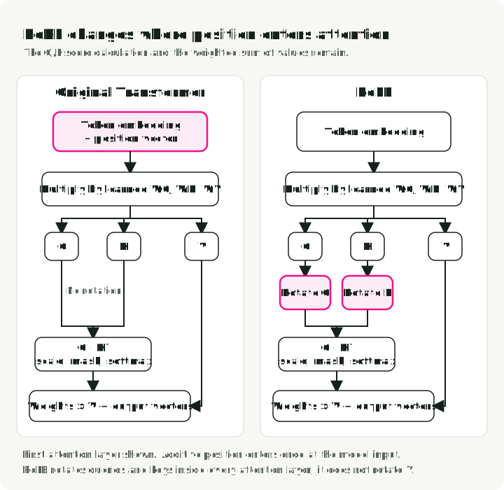
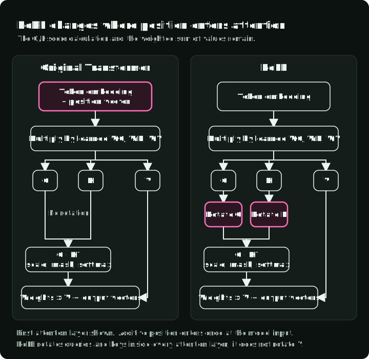
A query–key dot product compares content vectors. By itself, it does not say whether two tokens are adjacent or a hundred positions apart. The original Transformer adds a position vector to each token embedding before the first attention layer. Position information then influences the queries, keys and values computed from those inputs. It does not rotate them. See Attention Is All You Need, §3.5.

RoPE puts position into the query–key comparison itself. First compute the queries and keys with the usual learned projections. Then rotate pairs of their coordinates by angles determined by each token’s position. Compute the attention scores from those rotated vectors. Values are not rotated by RoPE.

The two panels below show where position enters. The weighted-value calculation remains after the score calculation in both cases.

$The original Transformer adds position to the input before forming queries, keys and values. RoPE rotates the projected queries and keys before their dot product, leaving values unrotated.$ $The original Transformer adds position to the input before forming queries, keys and values. RoPE rotates the projected queries and keys before their dot product, leaving values unrotated.$

For one coordinate pair, rotation is a matrix multiplication:

R(\varphi)=\begin{pmatrix} \cos\varphi&-\sin\varphi\\ \sin\varphi&\cos\varphi \end{pmatrix}.

$\varphi$ is the rotation angle. Multiplying this matrix by $(1,0)$ gives $(\cos\varphi,\sin\varphi)$ ; at 90° that is $(0,1)$ , the upward query arrow in the next diagram.

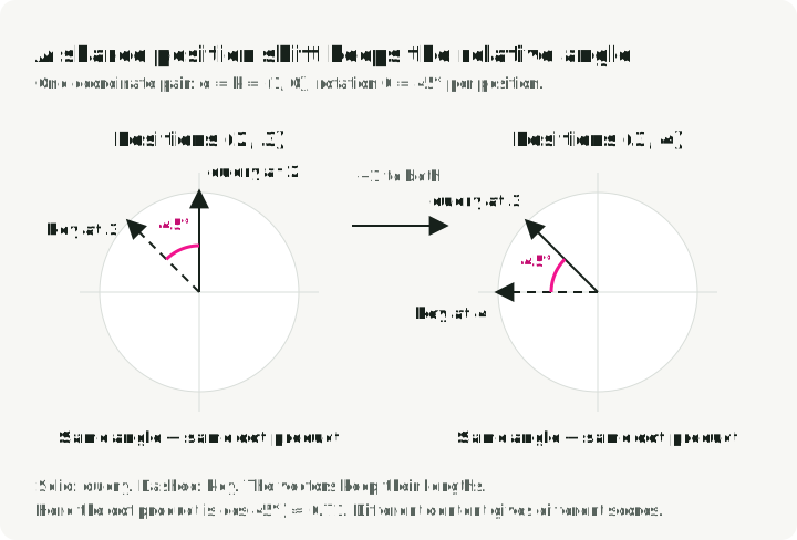
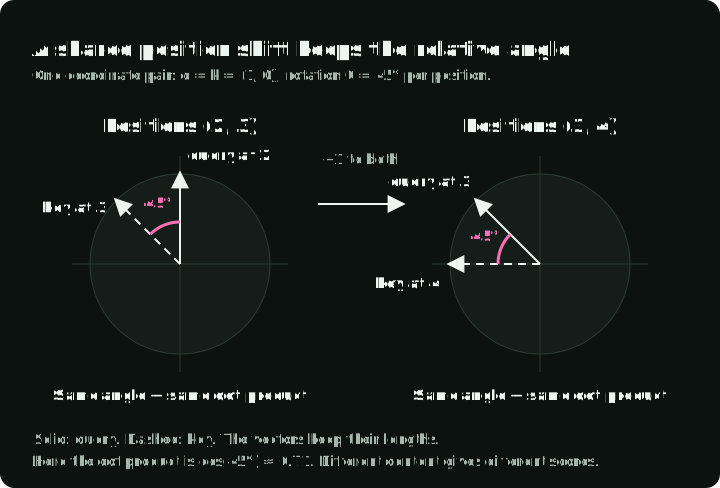
Why a rotation? A dot product depends on the angle between vectors. Rotating both vectors by the same extra angle leaves their dot product unchanged. If a query at position 2 and a key at position 3 move to positions 3 and 4, their position difference is still one. With the same underlying content vectors, RoPE gives the same score:

\begin{aligned} &\bigl(R(m\theta)q\bigr)^\top\bigl(R(n\theta)k\bigr)\\ &\qquad=q^\top R\bigl((n-m)\theta\bigr)k. \end{aligned}

Here $q$ and $k$ are one pair of query and key coordinates, $R$ rotates them, $m$ and $n$ are token positions, and $\theta$ is the rotation angle per position. The right-hand side exposes the useful property: the explicit position term uses the difference $n-m$ . The score still depends on the content vectors, not just the distance.

The diagram fixes both original vectors at $(1,0)$ and uses a rotation of 45° per position. These are chosen example values: holding content fixed lets us see the effect of shifting both positions.

$Two query–key pairs with the same underlying vectors and the same position difference. Shifting both positions rotates both arrows equally and preserves their angle and dot product.$ $Two query–key pairs with the same underlying vectors and the same position difference. Shifting both positions rotates both arrows equally and preserves their angle and dot product.$

A full query or key has many coordinate pairs. RoPE rotates them at different rates, so they represent position differences at several scales. That does not guarantee good attention at arbitrary context lengths, or that every score decreases with distance.

The rotation matrices and their derivation are in RoFormer v5, §3.2, equations (12)–(16). The detailed RoPE reading includes the intermediate algebra and numerical checks.

MLA: cache a small vector instead of keys and values

Attention heads existed before MLA. The original Transformer’s multi-head attention, §3.2.2, runs several attention calculations with different learned projections and combines their outputs. DeepSeek keeps multiple heads. Its change is how their keys and values are represented and cached.

During generation, ordinary multi-head attention stores a key and a value for each previous token for every head. This KV cache grows with the sequence. MLA instead uses a learned projection to turn the token’s incoming representation directly into one short vector. The heads’ content keys and values can be computed from it. All heads share this stored vector, but use different projections and attention weights; they do not become identical heads.

The diagram follows one token from its incoming vector to its stored data in one layer. Later queries read that data through multiple heads on both sides; the head outputs are combined into the attention output.

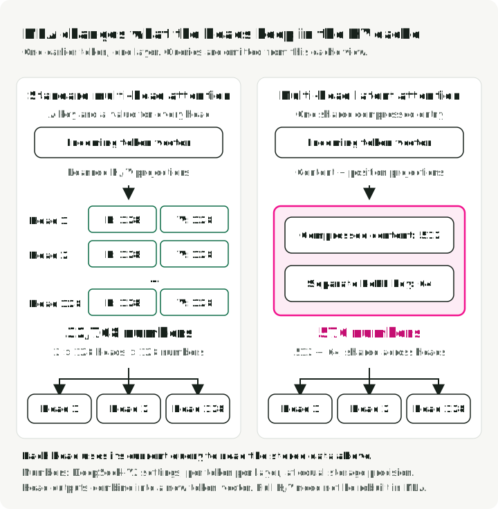
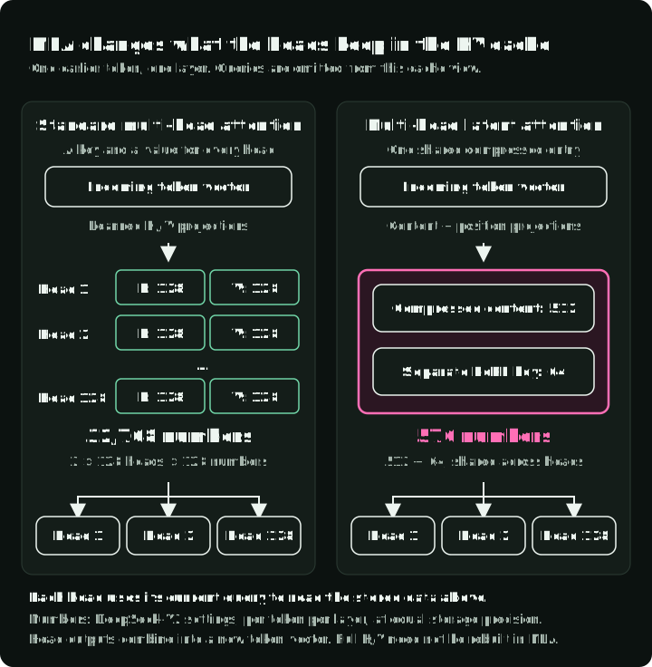
$Ordinary multi-head attention caches separate keys and values for every head. MLA caches one shared compressed vector and a separate small position key while retaining multiple attention heads.$ $Ordinary multi-head attention caches separate keys and values for every head. MLA caches one shared compressed vector and a separate small position key while retaining multiple attention heads.$

The content path in the diagram corresponds to three equations from DeepSeek-V2:

\begin{aligned} c_t^{KV}&=W^{DKV}h_t,\\ k_t^C&=W^{UK}c_t^{KV},\\ v_t^C&=W^{UV}c_t^{KV}. \end{aligned}

$h_t$ is token $t$ ‘s incoming vector. The first line maps it into the shorter cached vector $c_t^{KV}$ . The next two map that same vector into content keys and values for all heads. The superscripts are labels, not powers: $DKV$ names the down-projection, $UK$ and $UV$ name the key and value up-projections, and $C$ marks the content part. All three $W$ matrices are learned. The separate position key is outside these three equations.

For DeepSeek-V2’s configuration, the comparison is 32,768 numbers versus 576: ordinary attention with 128 heads and 128 numbers in each key and value needs $2\times128\times128$ ; MLA keeps a 512-number compressed vector and a 64-number position key. That is about 57 times fewer cached numbers at the same precision. It compares this configuration with ordinary multi-head attention, not every cache design, and does not imply 57 times faster inference.

Would expanding the compressed vector for every old token remove the benefit? MLA can avoid that expansion. For one head, shorten $c_t^{KV}$ to $c$ and call that head’s rows of $W^{UK}$ its key-expansion matrix $W_{\mathrm{up}}$ . Then:

q^\top(W_{\mathrm{up}}c)=(q^\top W_{\mathrm{up}})c.

The left side expands each cached vector into a key before comparing it with the query $q$ . The right side transforms the current query once, then compares it directly with the cached vectors. This is the same calculation grouped differently. The value calculation has a similar rearrangement: average the compressed vectors first, then apply the output projections. An implementation can choose the multiplication order that suits its hardware.

RoPE needs separate treatment. Rotating the expanded content keys would put a position-dependent operation inside that rearrangement. MLA therefore leaves those keys unrotated and adds a separate query–key comparison for position. That is why the cache contains both the compressed content vector and a small rotated position key.

MLA is a learned architecture, not a lossless compressor that can be applied to any existing attention layer. DeepSeek-V2 v5, §2.1.2–2.1.3, equations (9)–(19) defines the projections and the separate RoPE component. The detailed MLA reading gives the full shapes and matrix rearrangements.

Sparse attention (DSA): a cheap scorer picks the keys

DSA reduces how many tokens participate in each attention calculation. Suppose a model is continuing the text “The cat sat on a mat near me”. Treat each word as one token for this example. The model is processing the last token, “me”, at position 8.

Inside one attention layer, the current token’s representation produces a query vector. Each available token has a key, which the query is compared with, and a value, which supplies information to the output. During generation, the layer keeps earlier tokens’ attention data in its KV cache, so it can reuse those vectors. “Position 2” identifies the stored data for “cat”; the cache contains numerical vectors, not just position numbers. MLA stores this data in the compressed form described above.

Dense causal attention compares the current query with every available key, including the current token’s. Softmax converts those scores into weights, and the layer combines the values with those weights. DSA adds a cheaper selection step before that calculation:

Score the available tokens cheaply. A small learned network, the lightning indexer, uses its own query and key projections to score each position for the current token. It estimates which tokens the main attention will use most.
Select the highest-scoring positions. In the toy example, “cat” and “mat” receive the two largest index scores. Selecting positions 2 and 6 tells the main attention which stored entries to read.
Compute attention on those entries. The main attention computes its own query–key scores for the selected entries, applies softmax over that subset, and combines their values. The indexer’s scores choose the entries; they are not the final attention weights.

Follow a column from the text token to its stored entry, then compare the dense and sparse calculations. All scores and weights below are illustrative.

$Eight text tokens map to eight stored attention entries in one layer. The current token is “me”, at position 8. Dense attention uses all eight entries. DSA's separate indexer scores all positions and selects “cat” at position 2 and “mat” at position 6, with index scores 0.8 and 0.9. Main attention then computes new scores and softmax weights over those two entries; one illustrated head uses weights 0.7 and 0.3. The other cache entries remain stored.$ $Eight text tokens map to eight stored attention entries in one layer. The current token is “me”, at position 8. Dense attention uses all eight entries. DSA's separate indexer scores all positions and selects “cat” at position 2 and “mat” at position 6, with index scores 0.8 and 0.9. Main attention then computes new scores and softmax weights over those two entries; one illustrated head uses weights 0.7 and 0.3. The other cache entries remain stored.$

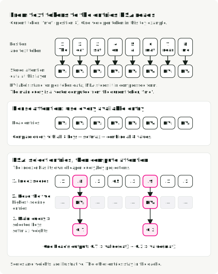
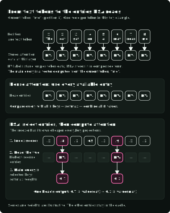
The paper’s indexer equation gives the first row of scores in the DSA panel:

I_{t,s}=\sum_{j=1}^{H^I}w^I_{t,j}\,\operatorname{ReLU}\bigl(q^I_{t,j}\cdot k^I_s\bigr).

$t$ is the current position and $s$ a candidate position. The superscript $I$ labels the indexer’s own vectors. For each of its $H^I$ heads, compare query $q^I_{t,j}$ with key $k^I_s$ , replace a negative dot product with zero using ReLU, multiply by the learned token-dependent weight $w^I_{t,j}$ , and sum over heads $j$ . The result $I_{t,s}$ is a selection score.

We can write the selection and one main-attention head’s output as:

\begin{aligned} \mathcal S_t&=\operatorname{TopKIndices}(I_{t,1:t},k),\\ u_t&=\sum_{s\in\mathcal S_t}a_{t,s}v_s. \end{aligned}

$I_{t,1:t}$ is the score row for available positions 1 through $t$ . TopKIndices returns the positions of its largest scores, up to $k$ entries. The sum reads “add the weighted values only for positions in $\mathcal S_t$ ”. Here $a_{t,s}$ is a newly computed main-attention softmax weight, $v_s$ its value vector, and $u_t$ the output. In the figure, $\mathcal S_8=\{2,6\}$ and $u_8=0.7v_2+0.3v_6$ . This rewrites the paper’s selected-entry notation as an explicit sum; MLA can calculate it in compressed form.

The other entries stay in the cache. A different query can select a different subset. Training teaches the indexer to approximate the main attention’s distribution over tokens, first with dense attention and then alongside sparse attention. A poor selection can omit useful information.

DeepSeek-V3.2 applies DSA to MLA’s compressed cache and selects up to 2,048 positions per query. At the final position of a 131,072-token context, the main attention reads one entry in 64. When fewer than 2,048 positions are available, it can use them all.

The saving comes from making fewer expensive attention comparisons. The indexer still scores every available position, but uses fewer heads and can compute in FP8. Across a sequence of length $L$ , the main attention’s comparisons fall from roughly $L^2$ to $Lk$ , where $k$ is the selected count. The indexer’s all-pairs work remains quadratic, so the whole method is not strictly linear in sequence length.

See DeepSeek-V3.2 v1, §2.1, equations (1)–(4) and the detailed DSA reading for the scoring and training equations.

Gated DeltaNet: a fixed-size memory that overwrites

Dense attention, MLA and DSA retain a growing record of past tokens. Gated DeltaNet instead updates one fixed-size matrix. The layer computes a key, value, and query from incoming token representations using learned projections and short filters over nearby tokens. The key and value update the matrix; the query reads the updated matrix to produce an output vector. It cannot separately revisit every old token’s key and value.

The useful comparison is with a simple additive memory. Suppose the memory currently returns 2 for a particular key, and the next token supplies value 5 for that same key. Adding the new value would produce 7. A delta update adds the correction, $5-2$ , so a full-strength write produces 5.

The example uses key $(1,0)$ , which reads the first column of the matrix: one times the first column plus zero times the second. The highlighted column shows the correction. After the write, a query $(1,0)$ reads $(5,0)$ from it. The matrix keeps the same size.

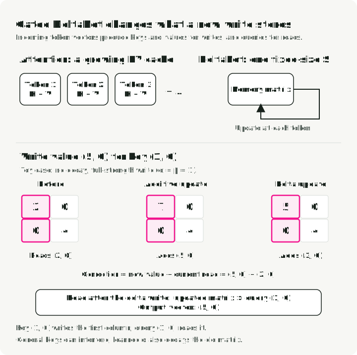
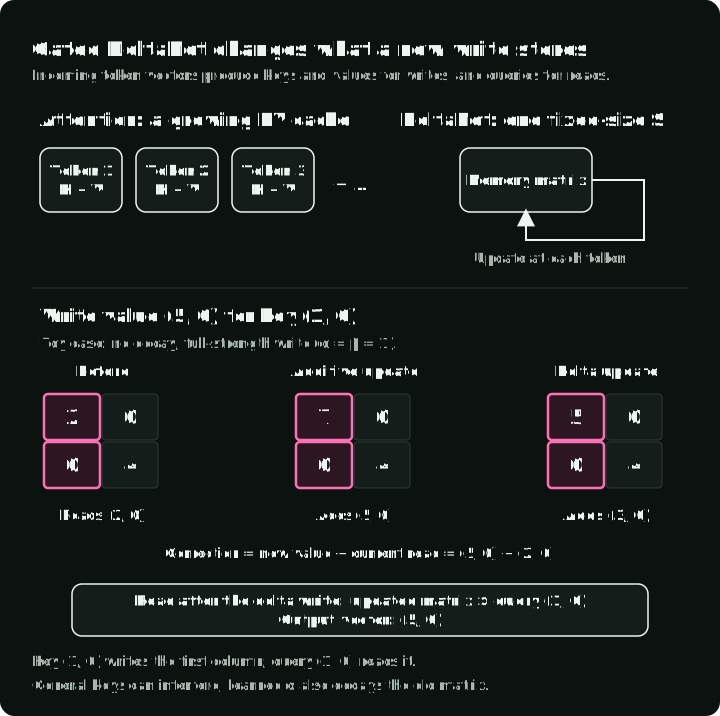
$Attention stores a growing KV cache, while DeltaNet updates a fixed-size matrix. Starting with diagonal entries 2 and 4, writing value (5, 0) for key (1, 0) gives first entry 7 under addition, or 5 under a delta correction. This example uses no decay and full write strength; general keys can affect other stored associations.$ $Attention stores a growing KV cache, while DeltaNet updates a fixed-size matrix. Starting with diagonal entries 2 and 4, writing value (5, 0) for key (1, 0) gives first entry 7 under addition, or 5 under a delta correction. This example uses no decay and full write strength; general keys can affect other stored associations.$

Gated DeltaNet also learns how much old memory to retain and how strongly to apply each correction:

S_t=\alpha_t S_{t-1}+\beta_t\bigl(v_t-\alpha_t S_{t-1}k_t\bigr)k_t^\top.

$S$ is the memory matrix, $k_t$ is the current unit-length key, and $v_t$ is its new value. The factor $\alpha_t$ decays the old memory. Reading the decayed memory with $k_t$ gives its current answer; subtracting that answer from $v_t$ gives the correction. The factor $\beta_t$ controls how much to write. Both factors are computed from the current token. Multiplying the updated matrix by the query gives the readout, which the layer then normalizes, gates, and projects into its output. The 2-to-5 example uses their limiting value of 1.

Fixed memory saves space, but writes can interfere: changing the answer for one key can change it for another non-orthogonal key. Decay also removes old information. This helps explain why the paper combines recurrent layers with sliding-window attention in hybrid models, retaining separate entries for recent tokens.

The displayed form rearranges Gated Delta Networks v3, §3.1, equation (10). The detailed reading derives it and works through the matrix update.

MoE routing: the bias picks experts, the score weights them

A mixture-of-experts (MoE) layer has several feed-forward networks, called experts, and selects only some for each token. This adds model capacity without running every expert for every input. It changes the feed-forward part of a Transformer, not its attention heads.

DeepSeek-V3’s particular routing rule separates two decisions: which experts run and how much their outputs count. A learned router takes the current token’s vector and gives each expert a score $s_i$ . A load-balancing bias $b_i$ changes the selection score to $s_i+b_i$ . After selection, the output weights come from the original scores, normalized over the selected experts. The bias does not enter those weights.

The toy example selects two of four experts. Expert 1 has the largest raw score, but its negative bias excludes it; experts 2 and 3 run instead. Both receive the same token vector $x$ . Each produces a new vector, written $E_2(x)$ or $E_3(x)$ , and the layer adds these outputs using weights 0.56 and 0.44. The diagram shows only this routed-expert contribution.

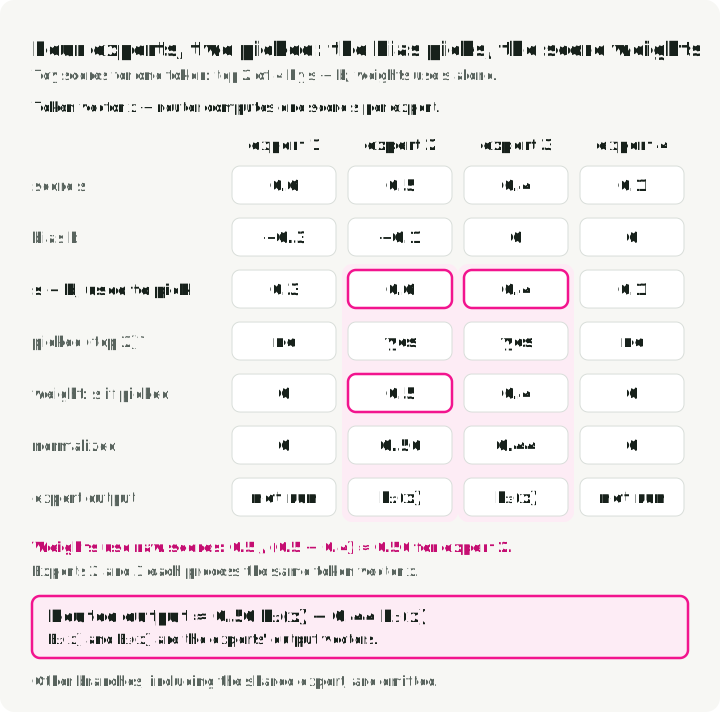
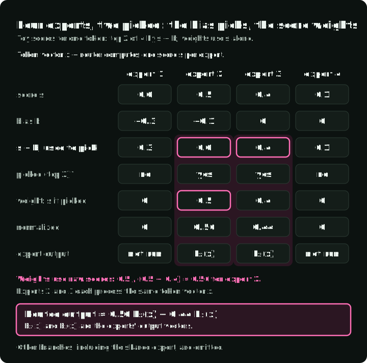
$Four experts are ranked by score plus bias to select experts 2 and 3. Their original scores, 0.5 and 0.4, determine output weights of about 0.56 and 0.44.$ $Four experts are ranked by score plus bias to select experts 2 and 3. Their original scores, 0.5 and 0.4, determine output weights of about 0.56 and 0.44.$

A compact form of DeepSeek-V3’s routing rule, for one token, is:

\begin{aligned} \mathcal E&=\operatorname{TopKIndices}(s+b,K),\\ g_i&=\begin{cases} \dfrac{s_i}{\sum_{j\in\mathcal E}s_j},&i\in\mathcal E,\\ 0,&i\notin\mathcal E, \end{cases}\\ u_{\mathrm{routed}}&=\sum_i g_iE_i(x). \end{aligned}

$s$ and $b$ collect all experts’ scores and biases; $K$ is the number to select. The first line returns the selected expert indices $\mathcal E$ . The brace in the second line is an if/else: divide a selected expert’s original score by the sum of selected scores, or assign zero if it was not selected. The last line adds the expert output vectors with these weights. In the figure, $\mathcal E=\{2,3\}$ , so $g_2=0.5/(0.5+0.4)\approx0.56$ and $g_3\approx0.44$ . The bias appears only in selection. The residual and shared-expert contributions are outside $u_{\mathrm{routed}}$ .

During training, an overused expert’s bias falls and an underused expert’s bias rises. This encourages a more even load. DeepSeek-V3 also retains a small per-sequence balancing loss, so “auxiliary-loss-free” does not mean the model has no balancing loss at all.

Its configuration activates 8 of 256 routed experts per token, plus one shared expert that always runs. Those counts and the shared expert belong to this model, not to the definition of MoE. See DeepSeek-V3 v2, §2.1.2, equations (12)–(17) and the routing reading.

mHC: residual mixing restricted to weighted averages

An ordinary residual connection carries a token vector past a sublayer and adds the sublayer’s result to it. mHC maintains several such vectors, called residual streams, and changes how they mix between layers. Its ideal mixing matrix has nonnegative entries with rows and columns summing to one. That mixing forms weighted averages while preserving the total across streams. The implementation approximates this constraint with a finite number of normalization steps; it does not constrain every operation in the network.

The separate mHC article explains the mechanism, normalization and limits with diagrams. Use it for that topic; the equation reading supplies the derivation.

LoRA: a low-rank update beside a frozen weight

Full fine-tuning updates the model’s weight matrices. LoRA freezes a pretrained matrix $W_0$ and learns a smaller correction alongside it:

h=W_0x+BAx.

$x$ is the token vector entering the chosen linear layer, and $h$ is the output vector passed onward through the model. The original multiplication $W_0x$ still runs. In the correction, $A$ maps the input into a much smaller vector, and $B$ maps it back to the output’s size. Training examples and the task loss determine updates to $A$ and $B$ ; $W_0$ stays fixed. Their shared small dimension is the rank setting $r$ ; the resulting update $BA$ has rank at most $r$ .

For a $4096\times4096$ weight matrix and $r=8$ , a full update has about 16.8 million entries. The two LoRA matrices have $4096\times8+8\times4096=65{,}536$ : 256 times fewer trainable entries for this matrix. That reduces gradient and optimizer-state storage, but the full base weight still occupies memory and participates in computation.

Follow the two paths from the same input: the frozen matrix still computes its output, while the trainable correction passes through just eight numbers.

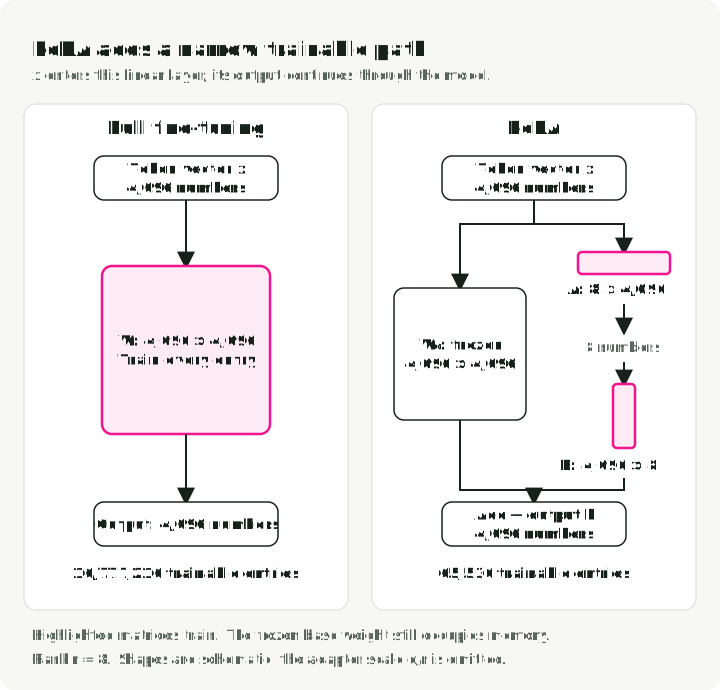
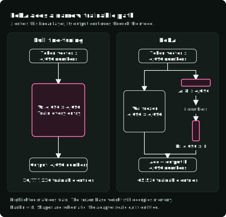
$Full fine-tuning trains all 16,777,216 entries of a 4096 by 4096 weight. LoRA freezes that weight and adds a parallel path through an 8 by 4096 matrix A and a 4096 by 8 matrix B. Their 65,536 entries train; the eight-number intermediate vector limits the correction's rank. Both paths produce 4096 numbers which are added.$ $Full fine-tuning trains all 16,777,216 entries of a 4096 by 4096 weight. LoRA freezes that weight and adds a parallel path through an 8 by 4096 matrix A and a 4096 by 8 matrix B. Their 65,536 entries train; the eight-number intermediate vector limits the correction's rank. Both paths produce 4096 numbers which are added.$

In the original method, $B$ starts at zero so the correction initially changes nothing. The paper scales the update by $\alpha/r$ , a setting omitted from its equation (3) above. After training, the scaled correction can be added to $W_0$ ; the merged layer then needs only the original matrix multiplication. Keeping adapters separate adds computation but allows them to be exchanged.

See LoRA v2, §4.1, equation (3) and the detailed LoRA reading. QLoRA additionally stores the frozen base weights in 4-bit form and dequantizes them for computation; it does not make all training memory 4-bit. The fine-tuning guide compares the practical options.

Optional equation walkthroughs

The linked equation readings contain symbol definitions, intermediate derivations and small-number checks. They were produced with the coding-agent instructions in paper-math-skills. They are supplementary explanations; the papers linked beside each mechanism are the primary sources.

Sources and versions

The paper links above identify the versions used for section and equation numbers. For the original attention baseline, see Attention Is All You Need v7, §3.2 and §3.5. For the separate residual-mixing topic, see mHC v2.