Reading the ELBO, diffusion loss, pass@k and scaling laws

This part explains what two generative models train and what four common measurements tell you. It is for engineers who want to understand the ELBO and diffusion loss, or compare papers reporting pass@k, perplexity, computational complexity and scaling laws. The diagrams show the computations; the equations identify exactly what is optimized or counted.
The generative-model sections build on each other. The metric sections can be read independently. Part 1 provides a notation reference if you need it. All logarithms here are natural logarithms.
Generative models: the ELBO and diffusion
A language model can assign a probability to a supplied answer one token at a time. Other generative models introduce hidden variables: intermediate values that help generate data but are absent from the training dataset. Computing an image’s probability can then require averaging over too many possible hidden values. The next two methods train without computing that average exactly.
ELBO: a lower bound you can compute
A variational autoencoder (VAE) generates an image from a latent vector : a list of numbers. A two-dimensional toy example is . These numbers are input to a neural network, not instructions in a programming language. The vector is latent because the training dataset contains images but does not supply their corresponding values.
To generate an image in the standard VAE described here, draw each entry of independently from a normal distribution with mean 0 and standard deviation 1. Drawing values according to a distribution is called sampling. This fixed distribution over vectors is the prior, written .
The decoder is a trained neural network. Its learned weights transform into the parameters of a distribution over pixel values. For example, a decoder for 28-by-28 images whose pixels are 0 or 1 can output 784 probabilities, one per pixel. Each probability gives the chance that its pixel is 1. Sampling those pixel values produces an image. The vector’s entries determine the pixel probabilities through the learned network; they are not themselves pixels. Kingma and Welling, §3 and Appendix C, describe this standard setup.
During training, an image comes from the dataset. An encoder, another neural network, takes this image as input. In the Gaussian setup used here, it predicts a mean and standard deviation for each entry of . Together these define , a distribution over latent vectors for this image. We sample from that distribution instead of the prior. The decoder then assigns probability to the original image using the sampled vector.
Training rewards the decoder for assigning a high log-probability to the observed image. It also subtracts KL divergence: a nonnegative measure of how much the encoder’s distribution over vectors differs from the fixed prior. The diagram shows both terms and the different source of vectors during generation.
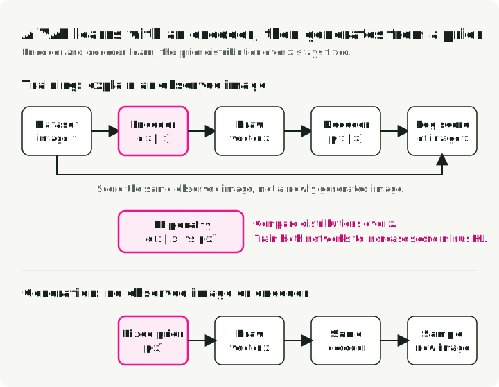
The training score has two terms:
The first term averages the image’s log-probability over vectors sampled from the encoder. The second is the KL penalty. The symbols and denote the encoder’s and decoder’s learned parameters. Both networks learn to increase this score; an implementation that minimizes a loss uses its negative.
This is the evidence lower bound, or ELBO. The evidence is the model’s probability for the observed image, averaged over all possible latent vectors. Kingma and Welling, §2.2, equations (1)–(3), relate it to the training score:
Here is the true posterior: the model’s distribution over latent vectors given this image. The nonnegative KL term is the gap between the ELBO and log-evidence; it is zero when the encoder matches that posterior. This identity explains the bound. The diagram’s computable training penalty instead compares the encoder with the known prior , so a training step does not require the unknown posterior.
A higher ELBO does not by itself prove that the decoder improved. A better encoder can make the bound more accurate while leaving the decoder unchanged. Also, the bound applies to the exact expectation: an estimate from a few sampled vectors can exceed the log-evidence on an individual draw. The detailed ELBO reading derives the bound and checks it with a worked example.
DDPM: predict the noise that was added
DDPM makes the hidden variables noisy versions of an image. During training, it takes a clean image from the dataset and draws random noise: one standard-normal number for each image coordinate. It randomly chooses a step from a fixed noise schedule, which sets the proportions of image and noise to mix. The network sees this corrupted image and ; its task is to predict the noise sample we just added.
Generation uses the trained network repeatedly. It starts from random noise, predicts noise at the current level, and uses that prediction to take a small denoising step. Its weights stay fixed during this process. Training therefore has a known target that supplies the error used to update the network; generation uses the learned network to produce an image through many steps.
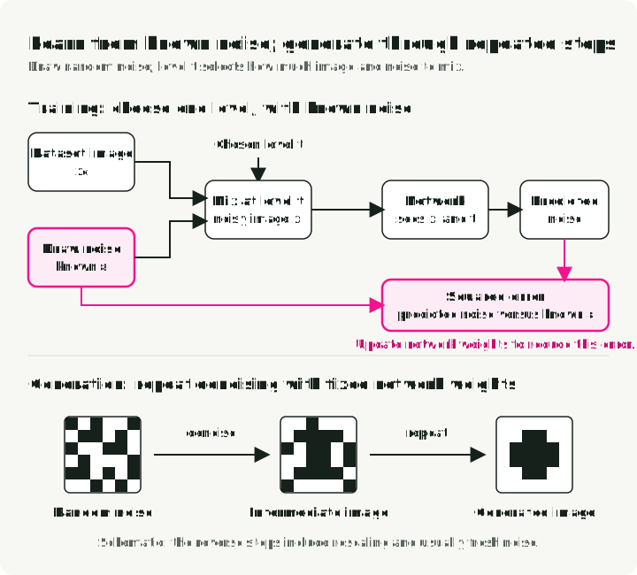
Writing the noisy input as makes the loss easier to read:
is a clean training image, is a randomly chosen step and is a fresh standard-normal noise sample. The network , with learned parameters , predicts that sample. The squared norm sums the squared prediction errors over image coordinates; the expectation averages over images, steps and noise samples.
The fixed schedule defines and , where is the noise variance added at step . The bar denotes this product, not an average. It sets the two coefficients in the diagram’s mixture: for the image and for noise. Near 1 means mostly image; near 0 means mostly noise.
Training can construct directly; it need not execute every preceding noise step. The original DDPM uses 1,000 levels and samples training steps uniformly. See equation (4), equation (14) and Algorithm 1, or the detailed DDPM reading.
The paper derives a variational bound related to the ELBO, then changes the weighting of its terms to obtain this practical loss. The simplified loss is not itself the original likelihood bound. During generation, Algorithm 2 rescales the current image, subtracts a multiple of predicted noise and, except at the last step, adds fresh noise. It does not simply subtract the prediction once to recover a clean image.
Metrics and cost claims
A training objective, an evaluation score and a cost estimate answer different questions. The next sections show what each reported number counts and what must stay fixed for a comparison to be useful.
Pass@k: the chance that at least one of k samples passes
pass@k asks whether at least one of generated programs passes the tests. It allows several attempts; it does not mean the model’s first answer is correct.
The Codex paper samples programs independently for each problem and counts the that pass. It then considers every possible set of samples. Subtract the fraction of sets that contain only failures:
The notation counts ways to choose items from without replacement. This is the estimate for one problem; the reported score averages it across problems. With five samples, two passing and three failing, there are ten pairs. Only three pairs contain two failures, so estimated pass@2 is .
The grid shows those ten pairs in this hypothetical example. All five programs answer the same problem and run against the same tests. A pair succeeds as soon as either of its two programs passes.
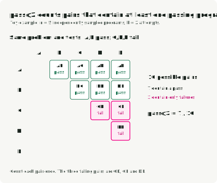
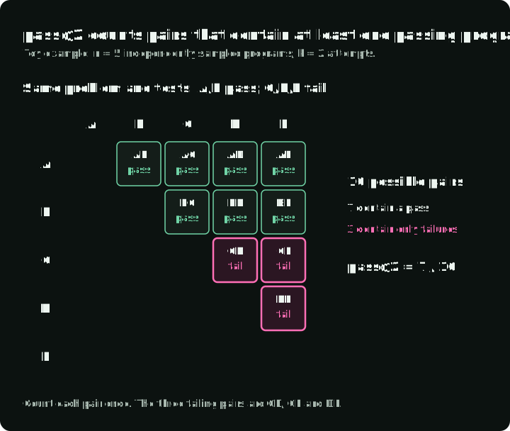
Use this estimator with integer counts and . If fewer than samples fail, every set contains a passing sample and the estimate is 1. The tempting shortcut is biased; it gives 0.64 in this example. The Codex paper, §2.1 and Figure 3, supplies the estimator and a numerically stable implementation; the detailed reading explains why it works.
Compare the same , problems, tests, prompts and generation settings. Passing the tests does not establish correctness for every input. A deployed system also needs a way to select a passing candidate, such as running those tests; merely generating several answers does not identify the good one.
Perplexity: the effective number of choices per token
Perplexity evaluates the probabilities a language model assigns to the actual next tokens of a supplied text. At each position, give the model the preceding text, obtain its probabilities over possible next tokens, and read the probability of the token that actually follows. No generated answer is needed. The score converts average negative log-probability into a more interpretable scale:
is the number of tokens, is the observed token and is its preceding context. If the model gives every observed token probability , perplexity is 4. If their probabilities differ, the score uses their geometric mean. Probabilities 0.5, 0.2 and 0.1 give perplexity about 4.64: the same score as assigning every token probability .
The charts use invented probabilities for three successive positions. Each bar comes from a different next-token prediction, so the bars do not need to sum to 1. The right chart replaces them with one constant value; the products match, so the perplexities match.
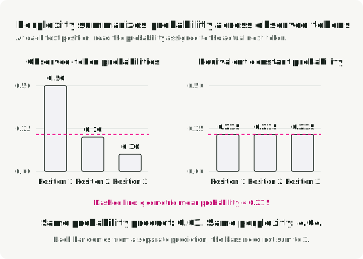
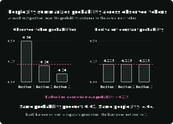
Lower is better for the same evaluation text, tokenizer and context procedure. It means the model assigned higher probability to the observed text, not that its generated answers are more useful or correct. Tokenizers split text differently, and context-window handling changes the probabilities. Hugging Face’s perplexity guide explains these comparison conditions.
Big-O: how cost grows with sequence length
Self-attention transforms each token’s current vector into a query, a key and a value using learned matrices. A query–key comparison scores how strongly one position should use another. These scores become weights for combining the values, as in the Transformer’s attention definition, §3.2.
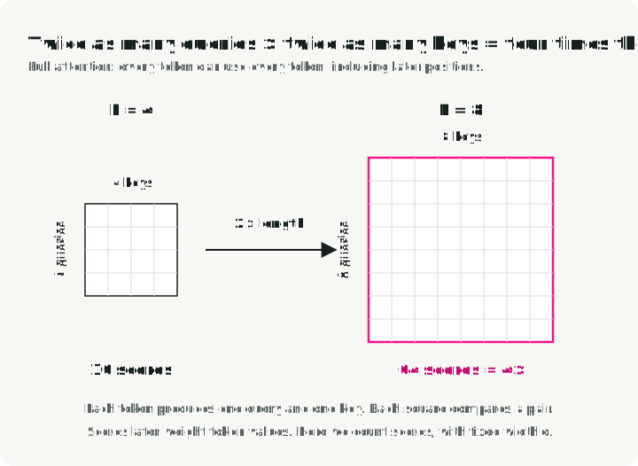
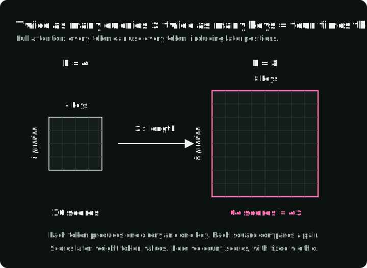
For one attention head and tokens, comparing every query with every key produces an score table. Doubling sequence length makes that table four times larger. If each comparison is a dot product of length , the score arithmetic grows as . Big-O describes an asymptotic upper bound; it omits constants and does not predict runtime by itself.
The grids show full attention: every position can use every position. A longer sequence adds both query rows and key columns. Each cell is one score; implementations such as FlashAttention can compute the scores without storing the whole grid at once. Causal attention excludes future positions, but its allowed-pair count still grows quadratically.
Different attention changes reduce different costs:
| Method | What changes | What still grows with the sequence |
|---|---|---|
| FlashAttention | Computes attention in blocks, avoiding a full score table in GPU main memory | Score arithmetic remains quadratic |
| DSA | A cheaper scorer selects up to tokens for full attention | The scorer still compares all eligible pairs |
| MLA | Stores less attention data per cached token | Cache size still grows linearly with token count |
These savings cannot be read as interchangeable speedups. Check whether a paper measured arithmetic, allocated memory, memory transfers or cache size. Also check whether it measured prompt processing or token generation; DeepSeek-V3.2, Figure 3, reports those phases separately.
Scaling laws: fitted curves with a valid range
A scaling law helps allocate a training budget between a larger model and more data. It is a curve fitted to experiments. For example, DeepSeek LLM, §3.2, equation (4), reports:
is training compute in floating-point operations. is non-embedding compute per token, used here as a measure of model size; it is not the parameter count. is the number of training tokens. The subscript “opt” marks the allocation fitted to minimize validation loss at that budget. The coefficients 0.1715 and 5.8316 belong to this fit and these units.
The curves below divide the fitted allocations by their values at a -FLOP budget, so each fitted coefficient cancels. A 100-fold budget increase gives times the compute per token and times the tokens. These are the two endpoints in the figure. Their factors multiply because the paper defines total compute as .
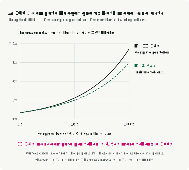
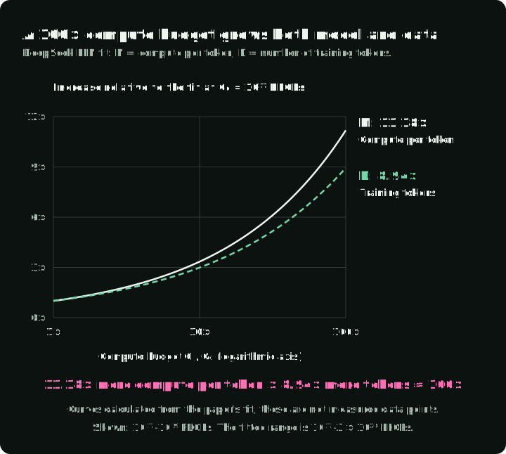
That conclusion belongs to these experiments. The fit covers to FLOPs. Outside that range it is an extrapolation; even inside it, different data or training settings can change the best allocation. Section 3.3 reports different exponents for different datasets. The detailed scaling-law reading explains the units and checks how the fitted formulas combine.
Reading an equation this series does not cover
For another equation, use Part 1’s six questions: identify the objects, operations, dimensions, sampling, learned quantities and claim being made.
The paper-math-skills repository provides agent instructions for writing and checking a detailed walkthrough. The linked readings are examples of that output, with symbol definitions and numerical checks.
Sources and versions
For a longer introduction to the foundations, see Tianhua Chen’s The Little Book of Generative AI Foundations, §3.2 for the ELBO.